
CMPUT-204 · Lesson 5 of 12 · 27 min
Sorting II: quicksort, heapsort and lower bounds
Merge sort is fast and predictable but needs a linear-size buffer. This lesson studies two in-place alternatives. Quicksort is usually the fastest comparison sort in practice, although its worst case is quadratic. Heapsort guarantees \(\Theta(n \log n)\) with constant extra space and introduces the binary heap, the priority queue behind Dijkstra's and Prim's algorithms in lessons 9 and 10. The lesson then proves that no comparison sort can beat \(\Theta(n \log n)\) in the worst case, and shows how counting sort and radix sort escape that bound by not comparing keys at all.
Partitioning
Quicksort is divide and conquer with the work done before the recursion instead of after. Choose an item called the pivot. Partition the array so that every item smaller than the pivot comes before it and every item larger comes after it. The pivot is now in its final position. Recursively sort the two sides; no combining step is needed. The Lomuto partition scheme scans the array once with an index \(i\) marking the end of the small region: each item smaller than the pivot is swapped into that region. Partitioning \(n\) items takes exactly \(n - 1\) comparisons.
Worked problem
Partitioning by hand
Partition 7, 2, 9, 4, 3, 8 using the last item, 8, as pivot (Lomuto).
Show solution
- Scan 7, 2, 9, 4, 3 and keep those smaller than 8 at the front: 7, 2, 4, 3 are smaller; 9 is larger.
- After the scan the array is 7, 2, 4, 3, 9, 8 with the small region 7, 2, 4, 3.
- Swap the pivot into the position after the small region: 7, 2, 4, 3, 8, 9.
- The pivot 8 is in its final position; recurse on 7, 2, 4, 3 and on 9.
Answer: 7, 2, 4, 3, 8, 9 with 8 fixed at index 4. Five comparisons were made, one per non-pivot item.
Quicksort's best, worst and expected cases
If every pivot splits its subarray into two halves, the recurrence is \(T(n) = 2T(n/2) + \Theta(n)\), the same as merge sort, so the best case is \(\Theta(n \log n)\). If every pivot is the smallest or largest item, one side is empty and the other has \(n - 1\) items, so \(T(n) = T(n-1) + \Theta(n)\), which unrolls to \(\Theta(n^2)\). With the last item as pivot, that disaster happens on input that is already sorted, a very common case in real data.
The cure is to choose the pivot uniformly at random. Then no particular input is bad; the running time is a random variable, and its expectation is \(\Theta(n \log n)\) for every input. A short proof counts comparisons: items \(z_i\) and \(z_j\), the \(i\)-th and \(j\)-th smallest, are compared only if one of them is the first pivot chosen from \(z_i, \ldots, z_j\), which happens with probability \(2/(j - i + 1)\). Summing over all pairs gives about \(2n \ln n \approx 1.39\, n \log_2 n\) expected comparisons. Randomized algorithms like this are a major topic in CMPUT-304; here it is enough to see that randomness turns a fragile algorithm into a reliable one.
import random, math

def quicksort(a, pivot_rule, counter):
    """Sort list a in place using Lomuto partitioning; count comparisons."""
    def part(lo, hi):
        if pivot_rule == 'random':
            k = random.randint(lo, hi)
            a[k], a[hi] = a[hi], a[k]
        p = a[hi]
        i = lo
        for j in range(lo, hi):
            counter[0] += 1
            if a[j] < p:
                a[i], a[j] = a[j], a[i]
                i += 1
        a[i], a[hi] = a[hi], a[i]
        return i
    stack = [(0, len(a) - 1)]            # explicit stack avoids deep recursion
    while stack:
        lo, hi = stack.pop()
        if lo < hi:
            m = part(lo, hi)
            stack.append((lo, m - 1)); stack.append((m + 1, hi))

random.seed(204)
n = 2000
for rule in ('last', 'random'):
    for name, data in (('random input', random.sample(range(n), n)), ('sorted input', list(range(n)))):
        c = [0]
        quicksort(data, rule, c)
        print(f'pivot={rule:<6} {name:<12} comparisons={c[0]:>8}')
print('n(n-1)/2 =', n * (n - 1) // 2, ' 1.39 n log2 n =', round(1.39 * n * math.log2(n)))pivot=last random input comparisons= 26332 pivot=last sorted input comparisons= 1999000 pivot=random random input comparisons= 25166 pivot=random sorted input comparisons= 22970 n(n-1)/2 = 1999000 1.39 n log2 n = 30485
With the last item as pivot, sorted input costs exactly \(n(n-1)/2\) comparisons, the quadratic worst case. With a random pivot, both inputs cost about 23,000 to 25,000 comparisons. The exact expectation is \(2(n+1)H_n - 4n\), roughly \(2n \ln n - 2.85n\), which is about 24,700 for \(n = 2000\); the leading term \(1.39\, n \log_2 n\) overstates the count for moderate \(n\) but describes its growth. In practice quicksort is fast because its inner loop is tiny and it scans memory sequentially, which caches reward. Production versions add refinements: the median of three items as pivot, insertion sort for small subarrays, three-way partitioning for many equal keys, and, in introsort, a switch to heapsort if the recursion gets too deep, which guarantees \(O(n \log n)\) in the worst case.
Binary heaps
A binary max-heap is a complete binary tree, filled level by level from the left, in which every node's key is at least as large as its children's keys. Because the tree is complete, it is stored in an array with no pointers: the children of index \(i\) are at \(2i + 1\) and \(2i + 2\), and its parent is at \(\lfloor (i-1)/2 \rfloor\). The heap property puts the maximum at the root, index 0, and the height of a heap with \(n\) items is \(\lfloor \log_2 n \rfloor\).
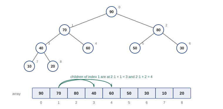
Two operations maintain the heap property. Sift-down repairs a node that may be smaller than a child: swap it with its larger child and repeat until it is larger than both children or becomes a leaf. Sift-up repairs a node that may be larger than its parent: swap upward until the parent is larger. Each walks one path of the tree, so each takes \(O(\log n)\) time. A priority queue supports insert (append, then sift up) and extract-max (move the last item to the root, then sift down) in \(O(\log n)\) each. Python's heapq module implements a min-heap the same way.
| Operation | Method | Time |
|---|---|---|
| Find maximum | Read index 0 | Θ(1) |
| Insert | Append at the end, sift up | O(log n) |
| Extract maximum | Move last item to root, sift down | O(log n) |
| Increase a key | Change it, sift up | O(log n) |
| Build heap from n items | Sift down every internal node, bottom up | Θ(n) |
Building a heap in linear time
Inserting \(n\) items one at a time costs \(O(n \log n)\). A faster method, due to Floyd, treats the array as a complete tree and sifts down each internal node, starting from the last one and moving toward the root. A node at height \(h\) costs \(O(h)\), and at most \(\lceil n/2^{h+1} \rceil\) nodes have height \(h\). Most nodes are near the bottom, where sifting is cheap, so the total is \(\sum_h \frac{n}{2^{h+1}} O(h) = O\!\left(n \sum_h \frac{h}{2^h}\right) = O(n)\), because \(\sum_h h/2^h = 2\). This is the geometric-series pattern from lesson 3 at work.
Heapsort
Heapsort builds a max-heap in \(\Theta(n)\) time, then repeatedly swaps the root, the largest remaining item, with the last item of the heap, shrinks the heap by one and sifts the new root down. After \(n - 1\) such steps the array is sorted in increasing order. Each step costs \(O(\log n)\), so heapsort takes \(O(n \log n)\) in the worst case and uses only \(O(1)\) extra space. It is not stable, and its jumps between parents and children make it cache-unfriendly, so it is usually slower than quicksort, but its guarantee makes it the safety net in introsort.
import random, math

def sift_down(a, i, n, counter):
    while True:
        l, r, big = 2 * i + 1, 2 * i + 2, i
        if l < n:
            counter[0] += 1
            if a[l] > a[big]: big = l
        if r < n:
            counter[0] += 1
            if a[r] > a[big]: big = r
        if big == i:
            return
        a[i], a[big] = a[big], a[i]
        i = big

def heapsort(a):
    build, sort = [0], [0]
    n = len(a)
    for i in range(n // 2 - 1, -1, -1):      # Floyd's bottom-up build
        sift_down(a, i, n, build)
    for end in range(n - 1, 0, -1):
        a[0], a[end] = a[end], a[0]
        sift_down(a, 0, end, sort)
    return build[0], sort[0]

random.seed(5)
for n in (1000, 10000, 100000):
    a = [random.random() for _ in range(n)]
    b, s = heapsort(a)
    assert a == sorted(a)
print(n, 'build:', b, round(b / n, 2), 'per item; sort phase:', s, round(s / (n * math.log2(n)), 2), 'x n log2 n')1000 build: 1825 1.82 per item; sort phase: 14993 1.5 x n log2 n 10000 build: 18873 1.89 per item; sort phase: 216595 1.63 x n log2 n 100000 build: 187884 1.88 per item; sort phase: 2831656 1.7 x n log2 n
The build phase uses under two comparisons per item for every size, confirming the linear bound, while the sort phase uses 1.5 to 1.7 times \(n \log_2 n\) comparisons, creeping toward 2 as \(n\) grows, because each sift-down step compares with both children. That constant is one reason quicksort, at about \(1.39\, n \log_2 n\), usually wins in practice.
A lower bound for comparison sorting
Can a cleverer comparison sort beat \(n \log n\)? No. Any comparison sort can be drawn as a decision tree: each internal node is a comparison of two keys, its two branches are the possible outcomes, and each leaf is the output permutation. Running the algorithm on an input traces one path from root to leaf, and the number of comparisons on that input is the path's length. The worst-case number of comparisons is the height of the tree.
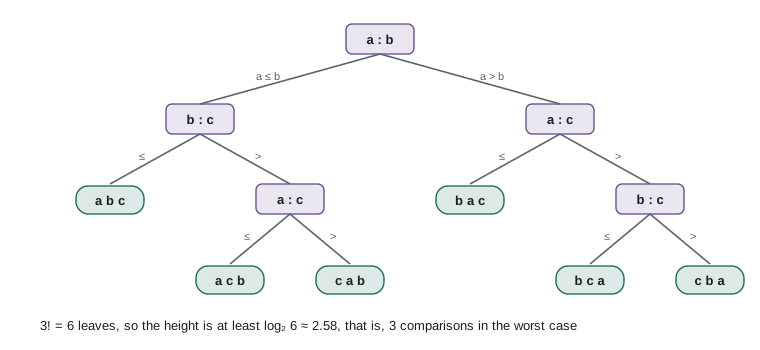
A correct sort must be able to produce each of the \(n!\) orderings of distinct keys, so the tree needs at least \(n!\) leaves. A binary tree of height \(h\) has at most \(2^h\) leaves, so \(2^h \ge n!\) and \(h \ge \log_2(n!)\). Since \(n! \ge (n/2)^{n/2}\), taking logarithms gives \(\log_2(n!) \ge \frac{n}{2}\log_2\frac{n}{2}\), which is \(\Omega(n \log n)\). Stirling's approximation sharpens this to \(\log_2(n!) \approx n \log_2 n - 1.44n\).
So merge sort and heapsort are asymptotically optimal among comparison sorts, and no amount of cleverness will change that. The argument is an information-theoretic one: each comparison yields one bit, and identifying one permutation out of \(n!\) needs \(\log_2(n!)\) bits. The same technique proves that searching a sorted list by comparisons needs \(\Omega(\log n)\) comparisons, so binary search is optimal too.
import math
for n in (3, 10, 100, 1000, 10**6):
    lb = math.lgamma(n + 1) / math.log(2)          # log2(n!) without computing n!
print(f'n={n:>7}: ceil(log2 n!) = {math.ceil(lb):>9}, n log2 n = {n * math.log2(n):>12.0f}, ratio {lb / (n * math.log2(n)):.3f}')n= 3: ceil(log2 n!) = 3, n log2 n = 5, ratio 0.544 n= 10: ceil(log2 n!) = 22, n log2 n = 33, ratio 0.656 n= 100: ceil(log2 n!) = 525, n log2 n = 664, ratio 0.790 n= 1000: ceil(log2 n!) = 8530, n log2 n = 9966, ratio 0.856 n=1000000: ceil(log2 n!) = 18488885, n log2 n = 19931569, ratio 0.928
Sorting in linear time without comparisons
The lower bound applies only to algorithms that learn about keys by comparing them. If keys are small integers, we can use them as array indices. Counting sort handles keys in the range 0 to \(k - 1\): count how many items have each key, compute running totals to find where each key's block starts, then place each item into the next free slot of its block, scanning the input from left to right so that equal keys keep their order and the sort is stable. It runs in \(\Theta(n + k)\) time and space, which is linear when \(k\) is \(O(n)\).
Radix sort extends this to larger keys by sorting on one digit at a time, starting with the least significant digit and using a stable sort such as counting sort for each pass. Stability is essential: after sorting by the tens digit, items with equal tens digits must stay in their order from the units pass. With \(d\) digits in base \(b\), radix sort takes \(\Theta(d(n + b))\) time. Sorting a million 32-bit integers as four base-256 digits takes four linear passes, which can beat a comparison sort's roughly 20 million comparisons.
def counting_sort_by(a, key, k):
    count = [0] * k
    for x in a:
        count[key(x)] += 1
    pos, total = [0] * k, 0
    for d in range(k):                   # starting index of each key's block
        pos[d], total = total, total + count[d]
    out = [None] * len(a)
    for x in a:                          # left-to-right with block starts keeps it stable
        out[pos[key(x)]] = x
        pos[key(x)] += 1
    return out

def radix_sort(a, base=10, digits=3):
    for d in range(digits):
        a = counting_sort_by(a, lambda x: (x // base ** d) % base, base)
        print(f'after digit {d}:', a)
    return a

radix_sort([329, 457, 657, 839, 436, 720, 355])after digit 0: [720, 355, 436, 457, 657, 329, 839] after digit 1: [720, 329, 436, 839, 355, 457, 657] after digit 2: [329, 355, 436, 457, 657, 720, 839]
Common mistakes
MistakeSaying quicksort is O(n log n) without qualification.
InsteadIts worst case is Θ(n²); with random pivots its expected time is Θ(n log n) on every input.
MistakeUsing the first or last item as pivot on data that may be sorted.
InsteadChoose a random pivot or the median of three to avoid the quadratic case on sorted input.
MistakeThinking building a heap by sifting down each node costs Θ(n log n).
InsteadMost nodes are near the bottom; the geometric sum gives Θ(n).
MistakeClaiming the n log n lower bound applies to every sorting algorithm.
InsteadIt applies to comparison sorts; counting and radix sort use keys as indices and run in linear time for small key ranges.
MistakeRunning radix sort with an unstable per-digit sort.
InsteadEach digit pass must be stable, or earlier passes are scrambled.
Summary and key terms
- Quicksort partitions around a pivot and recurses on both sides; partitioning n items takes n − 1 comparisons.
- Quicksort is Θ(n²) in the worst case, which a fixed pivot hits on sorted input, but random pivots give about 1.39 n log₂ n expected comparisons on every input.
- A binary heap is a complete tree stored in an array, with children of i at 2i + 1 and 2i + 2 and O(log n) insert and extract.
- Floyd's bottom-up heap construction runs in Θ(n) because most nodes are near the leaves.
- Heapsort sorts in place in O(n log n) worst-case time but is not stable.
- Every comparison sort needs at least log₂(n!) ∈ Ω(n log n) comparisons in the worst case, by the decision-tree argument.
- Counting sort and radix sort beat that bound by indexing on keys: Θ(n + k) and Θ(d(n + b)) respectively.
- Pivot
- The item around which quicksort partitions a subarray.
- Partition
- Rearranging a subarray so smaller items precede the pivot and larger items follow it.
- Randomized algorithm
- An algorithm that makes random choices, so its running time is a random variable.
- Binary heap
- A complete binary tree, stored in an array, in which each parent is at least (max-heap) or at most (min-heap) its children.
- Sift-down
- Swapping a node with its larger child until the heap property holds below it.
- Priority queue
- A data structure supporting insert and extract of the highest-priority item.
- Heapsort
- Build a max-heap, then repeatedly move the maximum to the end and sift down.
- Decision tree
- A tree representing every sequence of comparisons an algorithm can make on inputs of size n.
- Counting sort
- A stable sort for small integer keys that counts occurrences and places items by key.
- Radix sort
- Sorting by one digit at a time, least significant first, with a stable sort per digit.
Practice problems
Work each problem on paper first, then reveal the answer to check.
How many comparisons does quicksort make on sorted input of size 100 with the last item as pivot?
Show answer
100 × 99 / 2 = 4,950.
In an array heap, what are the children and parent of index 5?
Show answer
Children 11 and 12; parent ⌊4/2⌋ = 2.
What is the height of a heap with 1,000 items?
Show answer
⌊log₂ 1000⌋ = 9.
Is the array 9, 7, 8, 3, 5, 6, 4 a max-heap?
Show answer
Yes: 9 ≥ 7, 8; 7 ≥ 3, 5; 8 ≥ 6, 4.
What is the minimum worst-case number of comparisons to sort 4 distinct items?
Show answer
⌈log₂ 24⌉ = 5.
Why can counting sort beat the comparison lower bound?
Show answer
It never compares keys; it uses them as array indices, so the decision-tree model does not apply.
Radix sort 32-bit integers using base 65,536. How many passes?
Show answer
2 passes of 16 bits each.
Give the expected comparisons of random quicksort on 10⁶ items, roughly.
Show answer
1.39 × 10⁶ × 20 ≈ 28 million.
What does introsort do when quicksort recursion gets too deep?
Show answer
It switches to heapsort, guaranteeing O(n log n) worst-case time.
Why must the per-digit sort in radix sort be stable?
Show answer
So items with equal current digits keep the order established by less significant digits.
Lesson quiz · 5 questions
Score 60% or more to complete this lesson.
Create a free account to save your progress, take quizzes and earn a certificate.