
CMPUT-204 · Lesson 7 of 12 · 26 min
Graphs and graph search
Graphs model anything made of objects and connections: road networks, computer networks, web pages and links, course prerequisites, social networks and the states of a robot. CMPUT-272 lesson 12 introduced the vocabulary of graphs, degrees, paths and trees. This lesson turns to algorithms. It compares ways of storing a graph in memory and then develops the two fundamental ways of exploring one, breadth-first search and depth-first search. Both run in time linear in the size of the graph, and most of the graph algorithms in lessons 8 to 10 are built on top of them.
Graph vocabulary for algorithms
A graph \(G = (V, E)\) has a set \(V\) of vertices and a set \(E\) of edges. In an undirected graph an edge is an unordered pair \(\{u, v\}\); in a directed graph it is an ordered pair \((u, v)\) from \(u\) to \(v\). A weighted graph assigns each edge a number, such as a length or a cost. We write \(n = |V|\) and \(m = |E|\). An undirected simple graph has at most \(n(n-1)/2\) edges and a directed one at most \(n(n-1)\). A graph is sparse if \(m\) is close to \(n\), as in road networks where each intersection meets a handful of roads, and dense if \(m\) is close to \(n^2\).
Because graph sizes have two parameters, running times are expressed in both: \(\Theta(n + m)\), read linear in the size of the graph, is the best we can hope for when an algorithm must look at every vertex and edge. A path is a sequence of vertices joined by edges; its length is the number of edges, or the sum of weights in a weighted graph. An undirected graph is connected if there is a path between every pair of vertices, and its connected components are its maximal connected pieces.
Representing a graph
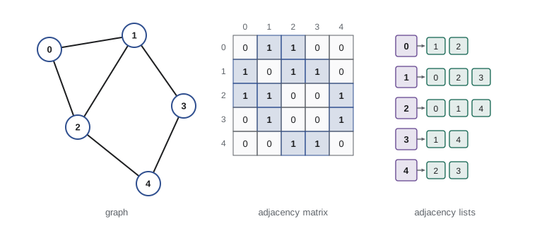
There are two standard representations. An adjacency matrix is an \(n \times n\) array whose entry in row \(u\), column \(v\) is 1, or the weight, if there is an edge from \(u\) to \(v\). An adjacency list stores, for each vertex, a list of its neighbours. In Python a dictionary of lists, or a list of lists indexed by vertex number, is natural; in C, the arrays-of-linked-lists or dynamic arrays from CMPUT-201 lesson 9 do the job.
| Operation | Adjacency matrix | Adjacency list |
|---|---|---|
| Space | Θ(n²) | Θ(n + m) |
| Is (u, v) an edge? | Θ(1) | Θ(deg u), or Θ(1) expected with hash sets |
| List neighbours of u | Θ(n) | Θ(deg u) |
| Visit every edge | Θ(n²) | Θ(n + m) |
| Add an edge | Θ(1) | Θ(1) |
| Best for | Dense graphs, fast edge tests | Sparse graphs, traversals |
Most real graphs are sparse, and most algorithms in this course spend their time listing neighbours, so adjacency lists are the default. A road network of Canada with a few million intersections would need trillions of matrix cells but only a few million list entries. The matrix wins when the graph is dense or when constant-time edge tests dominate, and it is the natural representation for algorithms built on matrix arithmetic. In an undirected graph each edge appears in two lists, so the lists hold \(2m\) entries; the handshaking lemma from CMPUT-272, \(\sum_v \deg(v) = 2m\), is exactly this count.
Breadth-first search
Breadth-first search, or BFS, explores a graph outward from a source vertex \(s\) in layers. It first visits \(s\), then all vertices one edge away, then all vertices two edges away, and so on. A first-in, first-out queue enforces the order: dequeue a vertex, look at each neighbour, and if the neighbour has not been seen, mark it, record its distance as one more than the current vertex's and its parent as the current vertex, and enqueue it. Each vertex enters the queue at most once and each adjacency list is scanned once, so BFS runs in \(\Theta(n + m)\) time with adjacency lists.
from collections import deque

def bfs(adj, s):
    dist = {s: 0}
    parent = {s: None}
    order = []
    q = deque([s])
    while q:
        u = q.popleft()
        order.append(u)
        for v in adj[u]:
            if v not in dist:              # first time seen: shortest distance found
                dist[v] = dist[u] + 1
                parent[v] = u
                q.append(v)
    return dist, parent, order

def path(parent, t):
    out = []
    while t is not None:
        out.append(t)
        t = parent[t]
    return out[::-1]

edges = [('A', 'B'), ('A', 'C'), ('B', 'D'), ('C', 'D'), ('C', 'E'), ('D', 'F'), ('E', 'F'), ('F', 'G')]
adj = {}
for u, v in edges:
    adj.setdefault(u, []).append(v)
    adj.setdefault(v, []).append(u)
dist, parent, order = bfs(adj, 'A')
print('visit order:', ' '.join(order))
print('distances  :', dict(sorted(dist.items())))
print('path A to G:', ' -> '.join(path(parent, 'G')))visit order: A B C D E F G
distances : {'A': 0, 'B': 1, 'C': 1, 'D': 2, 'E': 2, 'F': 3, 'G': 4}
path A to G: A -> B -> D -> F -> G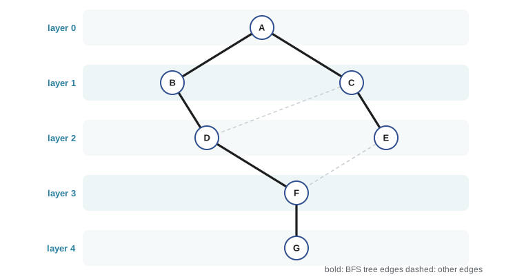
BFS computes shortest paths in unweighted graphs: when a vertex is first discovered, its recorded distance equals the minimum number of edges from \(s\). The proof uses an invariant on the queue: at all times, the distances of the vertices in the queue are non-decreasing from front to back and differ by at most 1. So vertices are dequeued in order of distance, and a vertex at distance \(k+1\) is discovered while processing some neighbour at distance \(k\), never later. The parent pointers form a BFS tree, and following them back from any vertex gives a shortest path.
Worked problem
Shortest path in a grid maze
A robot moves on a grid of open and blocked cells, one step up, down, left or right at a time. How can it find the fewest steps from start to goal?
Show solution
- Model each open cell as a vertex and each pair of adjacent open cells as an edge.
- Each vertex has at most 4 neighbours, so m ≤ 2n and the graph is sparse; neighbours can be computed on the fly with no stored list.
- Run BFS from the start cell; the first time the goal is dequeued, its distance is the minimum number of steps.
- Follow parent pointers back from the goal to recover the route.
Answer: BFS finds a fewest-steps route in Θ(n) time for n open cells. ROB-340 builds on this with weighted costs and heuristics such as A*.
Testing bipartiteness with BFS
A graph is bipartite if its vertices can be split into two groups with every edge going between the groups, for example jobs and workers, or students and courses. Equivalently, it can be coloured with two colours so that no edge joins two vertices of the same colour. BFS tests this in linear time: colour the source red, colour each newly discovered vertex the opposite colour of its parent, and check every edge. If some edge joins two vertices of the same colour, the graph is not bipartite. In fact, a graph is bipartite exactly when it has no cycle of odd length, and the BFS layers show why: an edge within one layer closes an odd cycle.
from collections import deque

def bipartition(adj):
    side = {}
    for s in adj:                          # handle every component
        if s in side:
            continue
        side[s] = 0
        q = deque([s])
        while q:
            u = q.popleft()
            for v in adj[u]:
                if v not in side:
                    side[v] = 1 - side[u]
                    q.append(v)
                elif side[v] == side[u]:
                    return None, (u, v)    # conflict: odd cycle
    return side, None

def make(edges):
    adj = {}
    for u, v in edges:
        adj.setdefault(u, []).append(v); adj.setdefault(v, []).append(u)
    return adj

square = make([(1, 2), (2, 3), (3, 4), (4, 1)])
triangle = make([(1, 2), (2, 3), (3, 1)])
for name, g in (('4-cycle', square), ('3-cycle', triangle)):
    c, bad = bipartition(g)
print(name, 'bipartite' if c else f'not bipartite, conflict on edge {bad}', dict(sorted(c.items())) if c else '')4-cycle bipartite {1: 0, 2: 1, 3: 0, 4: 1}
3-cycle not bipartite, conflict on edge (2, 3)Depth-first search
Depth-first search, or DFS, explores as far as possible along each branch before backing up. From the current vertex it moves to an unvisited neighbour and continues from there; when a vertex has no unvisited neighbours, the search returns to the vertex it came from. The natural implementation is recursive, so the call stack remembers the way back. DFS also runs in \(\Theta(n + m)\) time, because each vertex is visited once and each adjacency list is scanned once.
It is useful to record two timestamps for each vertex: the discovery time \(d[v]\), when the search first reaches \(v\), and the finish time \(f[v]\), when the search has explored everything reachable from \(v\) and returns from it. The intervals \([d[v], f[v]]\) are properly nested or disjoint, like parentheses, which is called the parenthesis theorem. Lesson 8 uses finish times to order the vertices of a directed acyclic graph and to find strongly connected components.
import sys
sys.setrecursionlimit(10000)

def dfs_all(adj):
    time = [0]
    d, f, parent = {}, {}, {}
    def visit(u):
        time[0] += 1; d[u] = time[0]
        for v in adj[u]:
            if v not in d:
                parent[v] = u
                visit(v)
        time[0] += 1; f[u] = time[0]
    for u in adj:                          # restart from every undiscovered vertex
        if u not in d:
            parent[u] = None
            visit(u)
    return d, f, parent

adj = {'A': ['B', 'C'], 'B': ['D'], 'C': ['D', 'E'], 'D': ['F'], 'E': ['F'], 'F': [], 'G': ['F']}
d, f, parent = dfs_all(adj)
for v in adj:
print(f'{v}: discovered {d[v]:>2}, finished {f[v]:>2}, parent {parent[v]}')A: discovered 1, finished 12, parent None B: discovered 2, finished 7, parent A C: discovered 8, finished 11, parent A D: discovered 3, finished 6, parent B E: discovered 9, finished 10, parent C F: discovered 4, finished 5, parent D G: discovered 13, finished 14, parent None
In the output, the search starts at A, goes deep through B, D and F, backs up, then explores C and E, and finally restarts at G, which nothing else reaches. F finishes first because it has no outgoing edges. Each interval is nested inside its ancestors' intervals: D's interval [3, 6] sits inside B's [2, 7], which sits inside A's [1, 12].
BFS or DFS?
| Property | BFS | DFS |
|---|---|---|
| Data structure | Queue | Stack (often the call stack) |
| Running time (lists) | Θ(n + m) | Θ(n + m) |
| Order of exploration | Layer by layer, by distance | Deep along one branch, then back up |
| Shortest paths (unweighted) | Yes | No |
| Discovery and finish times | Not naturally | Yes, used for ordering and components |
| Typical uses | Fewest-hops routes, bipartiteness, web crawling by depth | Topological sort, cycles, strongly connected components, maze generation |
| Memory risk | Wide graphs fill the queue | Deep graphs can overflow a recursion stack |
Both searches also solve simpler problems: deciding whether \(t\) is reachable from \(s\), and labelling connected components of an undirected graph by restarting the search from each unvisited vertex. For very deep graphs, a recursive DFS can exceed Python's recursion limit or overflow the C stack from CMPUT-201; an iterative version with an explicit stack avoids that, although recording finish times then needs a little more care.
Common mistakes
MistakeUsing an adjacency matrix for a large sparse graph.
InsteadA matrix needs Θ(n²) space and Θ(n²) time to scan; adjacency lists use Θ(n + m).
MistakeMarking a vertex visited when it is dequeued in BFS rather than when it is enqueued.
InsteadMark it when first discovered; otherwise it can be enqueued many times and distances can be wrong.
MistakeUsing DFS to find shortest paths in an unweighted graph.
InsteadDFS paths can be very long; BFS discovers vertices in order of distance.
MistakeSearching only from one source and concluding the graph has been explored.
InsteadRestart the search from every undiscovered vertex to cover all components.
MistakeSaying BFS runs in Θ(n²) on every graph.
InsteadWith adjacency lists it is Θ(n + m); it is Θ(n²) only with a matrix or a dense graph.
Summary and key terms
- A graph has n vertices and m edges; running times are written in both, and Θ(n + m) is linear in the size of the graph.
- Adjacency lists use Θ(n + m) space and suit sparse graphs; adjacency matrices use Θ(n²) space but answer edge queries in Θ(1).
- BFS uses a queue to explore in layers and runs in Θ(n + m).
- In an unweighted graph, BFS distances are shortest-path lengths and parent pointers give shortest paths.
- A graph is bipartite if and only if it has no odd cycle, which a BFS two-colour test detects in linear time.
- DFS explores deeply using a stack or recursion and records discovery and finish times that nest like parentheses.
- Restarting a search from each unvisited vertex labels connected components.
- Directed graph
- A graph whose edges are ordered pairs (u, v) from u to v.
- Sparse graph
- A graph with m close to n, far fewer than the maximum possible edges.
- Adjacency matrix
- An n × n array recording which pairs of vertices are joined.
- Adjacency list
- For each vertex, a list of its neighbours.
- Breadth-first search
- Exploring a graph in layers of increasing distance from a source, using a queue.
- BFS tree
- The tree formed by BFS parent pointers, containing a shortest path to each reachable vertex.
- Bipartite graph
- A graph whose vertices split into two groups with every edge between the groups.
- Depth-first search
- Exploring as far as possible along each branch before backtracking.
- Discovery and finish times
- The times DFS first reaches a vertex and finishes exploring from it.
- Connected component
- A maximal set of vertices in an undirected graph with paths between every pair.
Practice problems
Work each problem on paper first, then reveal the answer to check.
How much memory does an adjacency matrix need for 100,000 vertices at one byte per cell?
Show answer
10¹⁰ bytes, about 10 GB.
A sparse graph has 10⁶ vertices and 3 × 10⁶ undirected edges. How many entries do its adjacency lists hold?
Show answer
6 × 10⁶, two per edge.
What data structure gives BFS its layer-by-layer order?
Show answer
A first-in, first-out queue.
In BFS from s, vertex v gets distance 3. What does that mean?
Show answer
The shortest path from s to v has exactly 3 edges.
Is a 5-cycle bipartite?
Show answer
No: it is an odd cycle.
Is every tree bipartite?
Show answer
Yes: a tree has no cycles at all, so no odd cycles; colour vertices by the parity of their depth.
DFS gives d[u] = 3, f[u] = 10 and d[v] = 5, f[v] = 8. How are u and v related?
Show answer
v is a descendant of u in the DFS forest, since [5, 8] lies inside [3, 10].
How do you count connected components with BFS?
Show answer
Loop over vertices and start a new BFS from each unvisited one; count the starts.
Why might recursive DFS crash on a long path of a million vertices?
Show answer
The recursion depth would be a million, exceeding the stack or recursion limit.
What is the running time of BFS using an adjacency matrix?
Show answer
Θ(n²), since listing each vertex's neighbours scans a whole row.
Lesson quiz · 5 questions
Score 60% or more to complete this lesson.
Create a free account to save your progress, take quizzes and earn a certificate.