Nearest neighbours and decision trees

The linear models of the last three lessons make a strong assumption about the shape of the decision boundary. This lesson turns to two families that make almost none. A k-nearest-neighbour classifier stores the training data and labels a new point by a vote among the closest stored points. A decision tree asks a sequence of simple questions about the features, each splitting the data in two, until the remaining examples mostly share a label. Both are nonparametric in the sense that their complexity grows with the data rather than being fixed in advance, both handle multiple classes and regression with no change, and both are easy to explain to a non-specialist. They also illustrate, more vividly than any other methods, the bias–variance trade-off of lesson 2: each has a single knob, k or the tree depth, that moves it from memorizing the data to averaging it into a blur.

Decision trees matter for another reason: they are the building blocks of random forests and gradient-boosted trees, the subject of lesson 7, which are among the most accurate methods available for tabular data. Understanding how a single tree is grown and why it overfits is the first step to understanding why ensembles of them work so well.

The k-nearest-neighbour rule

Given a query point x, find the k training points closest to it under some distance, usually Euclidean, and predict the majority label among them (for classification) or their average target (for regression). There is no training phase beyond storing the data, which is why k-NN is called a lazy learner. The method goes back to Evelyn Fix and Joseph Hodges's 1951 technical report for the US Air Force School of Aviation Medicine, and Thomas Cover and Peter Hart proved in 1967 a famous guarantee: as the training set grows without bound, the error of the 1-nearest-neighbour rule is at most twice the Bayes error. With k growing too, but more slowly than n, the k-NN rule is consistent, meaning its error converges to the Bayes error for any distribution.

The choice of k sets the bias–variance trade-off. With k = 1, every training point owns a small region (its Voronoi cell), the decision boundary is jagged and follows every noisy label, and training error is zero. With k = n, every query gets the overall majority label. In between, larger k averages over more neighbours and gives smoother boundaries. A common practice is to choose k by cross-validation, using odd values for two classes to avoid ties; weighting neighbours by inverse distance is a frequent refinement.

# k-NN classification from scratch: the effect of k.
import numpy as np
rng = np.random.default_rng(367)
def moons(n, noise=0.3):
    a = rng.uniform(0, np.pi, n)
    upper = np.column_stack([np.cos(a), np.sin(a)])
    lower = np.column_stack([1 - np.cos(a), 0.5 - np.sin(a)])
    X = np.vstack([upper[: n // 2], lower[n // 2:]]) + rng.normal(0, noise, (n, 2))
    return X, np.r_[np.zeros(n // 2), np.ones(n - n // 2)].astype(int)
Xtr, ytr = moons(200); Xte, yte = moons(2000)

def knn_predict(Xtr, ytr, Xq, k):
    d2 = ((Xq[:, None, :] - Xtr[None, :, :]) ** 2).sum(axis=2)   # squared distances, queries x train
    idx = np.argsort(d2, axis=1)[:, :k]                          # indices of the k closest
    return (ytr[idx].mean(axis=1) > 0.5).astype(int)             # majority vote (k odd)

print("  k   train error   test error")
for k in (1, 3, 7, 15, 31, 75, 199):
    tr = np.mean(knn_predict(Xtr, ytr, Xtr, k) != ytr)
    te = np.mean(knn_predict(Xtr, ytr, Xte, k) != yte)
    print(f"{k:3}   {tr:11.3f}   {te:10.3f}")

  k   train error   test error
  1         0.000        0.118
  3         0.070        0.087
  7         0.065        0.089
 15         0.080        0.098
 31         0.095        0.119
 75         0.120        0.155
199         0.255        0.327

With k = 1 the classifier memorizes the training set, including its noise, and its test error is well above the best achievable. Moderate values of k cut the test error substantially. With k = 199, nearly the whole training set, every query receives almost the same vote, and the classifier collapses toward predicting a single class. Note also that the 1-NN training error of zero says nothing about its quality, a point lesson 1 made about memorizers in general.

Distance, scaling and cost

Everything about k-NN depends on the distance function. If one feature is income in dollars and another is age in years, Euclidean distance is almost entirely income, and age is ignored. Standardizing features (lesson 10) is therefore essential; better still, choose a distance that reflects what similar means for the problem: cosine similarity for text, edit distance for strings, or a learned metric. Irrelevant features are also harmful, because they add noise to every distance.

Prediction is expensive: a naive implementation computes the distance from the query to all n training points, costing O(nd) per query. Spatial index structures such as k-d trees and ball trees answer exact queries much faster in low dimensions, and approximate nearest neighbour methods such as locality-sensitive hashing and graph-based indexes (for example HNSW) make search over billions of vectors practical. These approximate indexes are the engine behind the vector databases used for retrieval with language models, which AI-410 describes.

The curse of dimensionality

Nearest neighbour methods rest on the assumption that the nearest training points are close, and in high dimensions they are not. Richard Bellman coined the phrase curse of dimensionality in 1957 for the explosive growth of volume with dimension. Two facts make it concrete. To capture a fixed fraction r of uniformly spread data in a cube neighbourhood in d dimensions, the cube's side must be \(r^{1/d}\): capturing 1 per cent of the data in 10 dimensions takes a cube spanning 63 per cent of each axis, hardly a local neighbourhood. And the distances from a query to random points concentrate: the nearest and farthest points become almost equally far away, so the idea of a nearest neighbour loses meaning.

# The curse of dimensionality: distances concentrate as the dimension grows.
import numpy as np
rng = np.random.default_rng(0)
print("  dim   nearest/farthest distance ratio   fraction of a unit cube within 0.1 of a face")
for d in (1, 2, 10, 100, 1000):
    X = rng.uniform(size=(500, d)); q = rng.uniform(size=d)
    dist = np.linalg.norm(X - q, axis=1)
    shell = 1 - 0.8 ** d                       # volume outside the inner cube [0.1, 0.9]^d
    print(f"{d:5}   {dist.min() / dist.max():33.3f}   {shell:44.3f}")

  dim   nearest/farthest distance ratio   fraction of a unit cube within 0.1 of a face
    1                               0.002                                          0.200
    2                               0.012                                          0.360
   10                               0.369                                          0.893
  100                               0.664                                          1.000
 1000                               0.903                                          1.000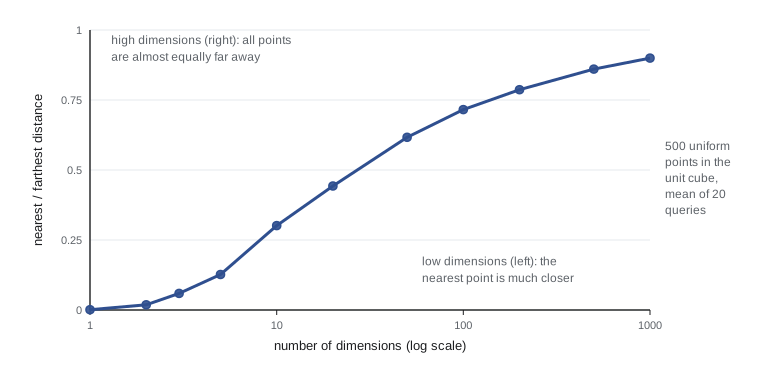

Real data are rarely uniform in their full space. Images, sounds and text occupy thin, curved regions (manifolds) of much lower intrinsic dimension than their raw representation, which is why nearest neighbour search on good learned embeddings works well even when the embeddings have hundreds of dimensions. The practical lessons are to reduce dimension (lesson 12), to select relevant features, or to learn a representation in which distance means something.

Decision trees

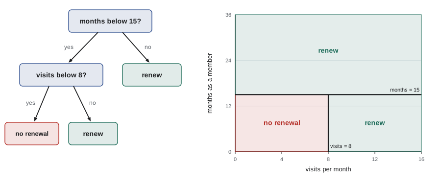
A decision tree is a flowchart. Each internal node tests one feature, typically asking whether a numeric feature is below a threshold or a categorical feature takes a particular value; each branch leads to another test or to a leaf, which holds a prediction. To classify an example, start at the root and follow the branches its feature values select. Geometrically, a tree with axis-aligned threshold tests partitions the input space into rectangular boxes and assigns each box a label. Trees handle mixed numeric and categorical features, need no feature scaling, ignore irrelevant features if they are never chosen for a split, and produce models a domain expert can read.

Finding the smallest tree consistent with the data is NP-hard, so trees are grown greedily from the top down. At each node, consider every feature and every candidate threshold, choose the split that most improves the purity of the two children, and recurse on each child until a stopping rule applies. Ross Quinlan's ID3 (1986) and C4.5 algorithms and the CART algorithm of Leo Breiman, Jerome Friedman, Richard Olshen and Charles Stone (1984) differ in details such as multiway versus binary splits and how they prune, but share this greedy recursive structure.

Measuring impurity

A node is pure if all its examples share a label. For a node in which a fraction \(p_k\) of examples belong to class k, two common impurity measures are the entropy and the Gini index:

Both are zero for a pure node and largest when classes are equally mixed (1 bit and 0.5, respectively, for two classes). The quality of a split is the decrease in impurity from parent to children, weighting each child by its share of examples. With entropy, this decrease is the information gain:

Information gain is the mutual information between the split and the label: how many bits the answer to the question tells us about the class. In practice entropy and Gini almost always choose the same splits. Misclassification rate is a poor splitting criterion, because many useful splits do not change the majority label in either child and so show zero improvement. For regression trees, the impurity is the variance of the targets in the node, and leaves predict the mean.

# A decision tree classifier from scratch (CART-style binary splits, entropy criterion).
import numpy as np
rng = np.random.default_rng(367)
# invented data: will a customer renew a gym membership?
n = 600
visits = rng.poisson(6, n)                 # visits per month
months = rng.integers(1, 37, n)            # months as a member
age = rng.integers(18, 70, n)
p = np.where(visits >= 8, 0.9, np.where(months >= 12, 0.65, 0.15))
y = (rng.uniform(size=n) < p).astype(int)
X = np.column_stack([visits, months, age]); names = ["visits", "months", "age"]

def entropy(y):
    if len(y) == 0: return 0.0
    q = np.mean(y)
    return 0.0 if q in (0, 1) else -(q * np.log2(q) + (1 - q) * np.log2(1 - q))

def best_split(X, y):
    best = (0.0, None, None)
    for j in range(X.shape[1]):
        for t in np.unique(X[:, j])[1:]:              # candidate thresholds: observed values
            left = X[:, j] < t
            gain = entropy(y) - (left.mean() * entropy(y[left]) + (~left).mean() * entropy(y[~left]))
            if gain > best[0]: best = (gain, j, t)
    return best

def grow(X, y, depth, max_depth, min_leaf=5):
    gain, j, t = best_split(X, y)
    if depth == max_depth or j is None or gain < 0.02 or len(y) < 2 * min_leaf:
        return {"leaf": int(round(np.mean(y))), "n": len(y), "p": round(float(np.mean(y)), 2)}
    left = X[:, j] < t
    return {"f": j, "t": t, "gain": gain, "L": grow(X[left], y[left], depth + 1, max_depth),
            "R": grow(X[~left], y[~left], depth + 1, max_depth)}

def show(node, depth=0, branch=""):
    pad = "    " * depth + branch
    if "leaf" in node:
        print(f"{pad}predict {node['leaf']}  (n={node['n']}, P(renew)={node['p']})"); return
    print(f"{pad}{names[node['f']]} < {node['t']}?  (gain {node['gain']:.3f} bits)")
    show(node["L"], depth + 1, "yes: "); show(node["R"], depth + 1, "no:  ")

show(grow(X, y, 0, max_depth=2))

months < 15?  (gain 0.129 bits)
    yes: visits < 8?  (gain 0.224 bits)
        yes: predict 0  (n=193, P(renew)=0.21)
        no:  predict 1  (n=57, P(renew)=0.84)
    no:  visits < 8?  (gain 0.039 bits)
        yes: predict 1  (n=266, P(renew)=0.72)
        no:  predict 1  (n=84, P(renew)=0.93)

The tree recovers the structure we built into the data, though not in the order we wrote it. We generated the labels by asking first about visits and then about months, but the greedy search puts months at the root, because that single split happens to reduce entropy most, and then asks about visits on each side. Its threshold of 15 months rather than 12 reflects noise in 600 examples. On the long-standing side, the visits split separates renewal probabilities of 0.72 and 0.93 but leaves both predicting renewal, which a pruning step would merge. Age, which played no role in generating the labels, is never chosen. Even this small example shows the main attraction of trees: the model can be read aloud as a set of rules.

Overfitting and pruning

Grown without limit, a tree keeps splitting until every leaf is pure, which on noisy data means a leaf for nearly every training example: zero training error, high variance and poor generalization. There are two remedies. Pre-pruning stops growth early, with a maximum depth, a minimum number of examples per leaf or split, or a minimum impurity decrease. Post-pruning grows a large tree and then cuts it back. CART's cost-complexity pruning minimizes \(\text{error}(T) + \alpha \lvert T \rvert\), where \(\lvert T \rvert\) is the number of leaves, over subtrees T of the full tree; increasing \(\alpha\) produces a nested sequence of smaller trees, and cross-validation chooses \(\alpha\). Post-pruning tends to work better because a split that looks useless on its own can enable valuable splits below it.

# Tree depth versus training and test error (scikit-learn's CART), and cost-complexity pruning.
import numpy as np
from sklearn.tree import DecisionTreeClassifier
rng = np.random.default_rng(8)
def make(n):
    X = rng.uniform(-1, 1, (n, 5))
    y = ((X[:, 0] ** 2 + X[:, 1] ** 2 < 0.5) ^ (rng.uniform(size=n) < 0.15)).astype(int)   # 15% label noise
    return X, y
Xtr, ytr = make(500); Xte, yte = make(5000)
print("max depth  leaves  train error  test error")
for d in (1, 2, 4, 6, 10, None):
    t = DecisionTreeClassifier(max_depth=d, random_state=0).fit(Xtr, ytr)
    print(f"{str(d):>9}  {t.get_n_leaves():6}  {1 - t.score(Xtr, ytr):11.3f}  {1 - t.score(Xte, yte):10.3f}")
full = DecisionTreeClassifier(random_state=0).fit(Xtr, ytr)
alphas = full.cost_complexity_pruning_path(Xtr, ytr).ccp_alphas
for a in (alphas[len(alphas) // 2], alphas[-8]):
    t = DecisionTreeClassifier(ccp_alpha=a, random_state=0).fit(Xtr, ytr)
    print(f"pruned with alpha={a:.4f}: {t.get_n_leaves()} leaves, test error {1 - t.score(Xte, yte):.3f}")

max depth  leaves  train error  test error
        1       2        0.418       0.472
        2       4        0.300       0.346
        4      13        0.190       0.253
        6      37        0.112       0.257
       10      84        0.020       0.282
     None      99        0.000       0.287
pruned with alpha=0.0032: 42 leaves, test error 0.260
pruned with alpha=0.0046: 15 leaves, test error 0.228

A depth-1 tree (a decision stump) underfits the circular boundary. Test error falls to a minimum at a moderate depth and rises again as the tree grows into the 15 per cent label noise; the fully grown tree has zero training error and one of the worst test errors. Pruning the full tree with a well-chosen \(\alpha\) gives a tree of 15 leaves whose test error is lower than that of any depth-limited tree in the table, still some way above the Bayes error of 0.15 set by the label noise.

Strengths and weaknesses of trees

Single trees are interpretable, fast, insensitive to monotone transformations of features (only the order of values matters), robust to outliers in the inputs and naturally handle interactions between features. Their weaknesses are just as characteristic. They are unstable: a small change in the training data can change the root split and hence the whole tree, which is high variance in its purest form. Axis-aligned splits approximate diagonal boundaries with staircases. And their accuracy is usually below that of a well-tuned linear model, SVM or ensemble. Lesson 7 turns the instability into an advantage: averaging many different trees cancels much of their variance.

Worked examples