Evaluating and comparing models

A model is only as good as the evidence that it works. This lesson is about producing that evidence honestly: estimating how well a model will do on new data, choosing measures of performance that reflect what the application needs, and deciding whether one model is really better than another or merely got luckier on a particular test set. These questions are where most published and deployed machine learning goes wrong, far more often than in the choice of algorithm. The techniques are simple; the discipline to apply them consistently is the hard part.

Hold-out estimates and their uncertainty

Lesson 1 introduced the basic protocol: fit on training data, choose on validation data, and estimate once on test data. A test-set error rate is itself an estimate, with sampling error. With m test examples and true error p, the observed error has standard deviation about \(\sqrt{p(1-p)/m}\), so 500 test examples and an error near 20 per cent give a standard error of about 1.8 percentage points and a 95 per cent interval of roughly plus or minus 3.5 points. Always report an interval, or at least the test set size, alongside a single number. A difference of one point between two models on a 500-example test set is noise.

Cross-validation

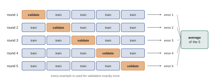
With limited data, a single split wastes examples and gives a noisy estimate that depends on which examples happened to land in the validation set. k-fold cross-validation uses all the data for both purposes. Divide the data at random into k folds of roughly equal size. For each fold in turn, train on the other k − 1 folds and evaluate on the held-out fold. Average the k error estimates. Each example is used for validation exactly once and for training k − 1 times. Common choices are k = 5 or 10; leave-one-out cross-validation (k = n) is nearly unbiased but expensive and has high variance, except for models like ridge regression and k-NN where it can be computed cheaply in closed form.

# k-fold cross-validation from scratch, used to choose k for k-NN.
import numpy as np
rng = np.random.default_rng(367)
def moons(n, noise=0.3):
    a = rng.uniform(0, np.pi, n)
    X = np.vstack([np.column_stack([np.cos(a[: n // 2]), np.sin(a[: n // 2])]),
                   np.column_stack([1 - np.cos(a[n // 2:]), 0.5 - np.sin(a[n // 2:])])])
    return X + rng.normal(0, noise, (n, 2)), np.r_[np.zeros(n // 2), np.ones(n - n // 2)].astype(int)
X, y = moons(300); Xte, yte = moons(5000)

def knn(Xtr, ytr, Xq, k):
    d2 = ((Xq[:, None] - Xtr[None]) ** 2).sum(axis=2)
    return (ytr[np.argsort(d2, axis=1)[:, :k]].mean(axis=1) > 0.5).astype(int)

def kfold_error(X, y, k_nn, folds=10):
    idx = rng.permutation(len(y)); parts = np.array_split(idx, folds)
    errs = []
    for f in range(folds):
        va = parts[f]; tr = np.concatenate([parts[g] for g in range(folds) if g != f])
        errs.append(np.mean(knn(X[tr], y[tr], X[va], k_nn) != y[va]))
    return np.mean(errs), np.std(errs) / np.sqrt(folds)

print("  k   10-fold CV error (± s.e.)   test error on 5,000 new points")
for k in (1, 5, 15, 45, 135):
    m, se = kfold_error(X, y, k)
    print(f"{k:3}   {m:.3f} ± {se:.3f}              {np.mean(knn(X, y, Xte, k) != yte):.3f}")

  k   10-fold CV error (± s.e.)   test error on 5,000 new points
  1   0.107 ± 0.018              0.136
  5   0.100 ± 0.021              0.102
 15   0.100 ± 0.015              0.092
 45   0.113 ± 0.020              0.108
135   0.153 ± 0.025              0.176

The cross-validation errors track the test errors on 5,000 fresh points closely, and both identify the same region of good values of k. The standard errors are a reminder that the differences between neighbouring choices are often within noise; a common heuristic, the one-standard-error rule, picks the simplest model whose cross-validation error is within one standard error of the best, here a larger k.

Several variations matter in practice. Stratified cross-validation keeps the class proportions the same in every fold, which matters for imbalanced data. Grouped cross-validation keeps all examples from one patient, customer or device in the same fold, so the model is evaluated on unseen groups, which is usually what deployment requires. Time-series cross-validation (forward chaining) always trains on the past and validates on the future, never the reverse. Choosing the wrong scheme is one of the commonest ways to get an optimistic estimate.

Nested cross-validation

Cross-validation is also the standard tool for choosing hyperparameters: try each candidate setting, pick the one with the lowest cross-validation error. But the cross-validation error of the winning setting is then optimistically biased, because it was selected for being low, exactly as a test error would be if used for selection. When an unbiased estimate of the whole procedure (including the hyperparameter search) is needed and data are too scarce for a separate test set, use nested cross-validation: an outer loop of folds estimates performance, and inside each outer training set an inner cross-validation chooses the hyperparameters. The outer estimate then evaluates the procedure, search included, on data the search never saw.

The confusion matrix

For classification, the error rate hides what kinds of mistakes a model makes. The confusion matrix counts, for a binary problem, true positives (TP), false positives (FP), false negatives (FN) and true negatives (TN). From it come the standard measures:

Accuracy is misleading when classes are imbalanced. If 2 per cent of transactions are fraudulent, a model that never flags anything is 98 per cent accurate and completely useless. Precision and recall focus on the positive class, which is usually the one that matters. They trade off against each other through the decision threshold: lowering the threshold flags more cases, raising recall and usually lowering precision.

# Confusion matrix, precision, recall, F1, ROC AUC and average precision, computed from scratch.
import numpy as np
from sklearn.metrics import roc_auc_score
rng = np.random.default_rng(367)
# invented scores from a fraud model: 2% of 10,000 transactions are fraudulent
n = 10_000; y = (rng.uniform(size=n) < 0.02).astype(int)
score = rng.normal(np.where(y == 1, 1.8, 0.0), 1.0)          # frauds score higher on average

def confusion(y, pred):
    tp = np.sum((pred == 1) & (y == 1)); fp = np.sum((pred == 1) & (y == 0))
    fn = np.sum((pred == 0) & (y == 1)); tn = np.sum((pred == 0) & (y == 0))
    return tp, fp, fn, tn

print("threshold   TP    FP   FN     TN  accuracy  precision  recall    F1")
for t in (1.0, 2.0, 3.0, 99):
    tp, fp, fn, tn = confusion(y, (score >= t).astype(int))
    prec = tp / (tp + fp) if tp + fp else 0.0; rec = tp / (tp + fn)
    f1 = 2 * prec * rec / (prec + rec) if prec + rec else 0.0
    print(f"{t:9}  {tp:3} {fp:5} {fn:4} {tn:6}  {(tp + tn) / n:8.3f}  {prec:9.3f}  {rec:6.3f}  {f1:5.3f}")

# ROC AUC as a probability: P(score of a random fraud > score of a random legitimate case)
order = np.argsort(score); ranks = np.empty(n); ranks[order] = np.arange(1, n + 1)
n1, n0 = y.sum(), n - y.sum()
auc = (ranks[y == 1].sum() - n1 * (n1 + 1) / 2) / (n1 * n0)
print(f"ROC AUC from ranks {auc:.4f}; scikit-learn {roc_auc_score(y, score):.4f}")
# average precision: mean precision at the rank of each fraud, scanning from the top score down
yy = y[np.argsort(-score)]; prec_at = np.cumsum(yy) / np.arange(1, n + 1)
print(f"average precision {np.sum(prec_at * yy) / n1:.3f}   (a random ranking would give about {y.mean():.3f})")

threshold   TP    FP   FN     TN  accuracy  precision  recall    F1
      1.0  178  1511   45   8266     0.844      0.105   0.798  0.186
      2.0   95   229  128   9548     0.964      0.293   0.426  0.347
      3.0   24    12  199   9765     0.979      0.667   0.108  0.185
       99    0     0  223   9777     0.978      0.000   0.000  0.000
ROC AUC from ranks 0.9065; scikit-learn 0.9065
average precision 0.306   (a random ranking would give about 0.022)

The never-flag rule (threshold 99) is 97.8 per cent accurate, almost the best accuracy in the table, and catches no fraud at all. At threshold 1.0 the model catches most frauds but buries them among many false alarms; at 3.0 its flags are more trustworthy but it misses most frauds. Which operating point is right depends on the costs: an investigator's time per false alarm against the loss per missed fraud. The F1 score, which weighs precision and recall equally, is a convenient summary but encodes an arbitrary cost ratio; when real costs are known, choose the threshold that minimizes expected cost, as in the decision rule of lesson 8.

ROC curves and AUC

A receiver operating characteristic (ROC) curve, a tool from signal detection in the Second World War, plots the true positive rate against the false positive rate as the threshold sweeps from high to low. A random scorer traces the diagonal; a perfect one hugs the top-left corner. The area under the curve (AUC) summarizes ranking quality in one number with a clean interpretation: it is the probability that a randomly chosen positive example receives a higher score than a randomly chosen negative one. That makes it equivalent to the Mann–Whitney U statistic, which is how the program computes it from ranks. AUC is independent of the threshold and of the class proportions.

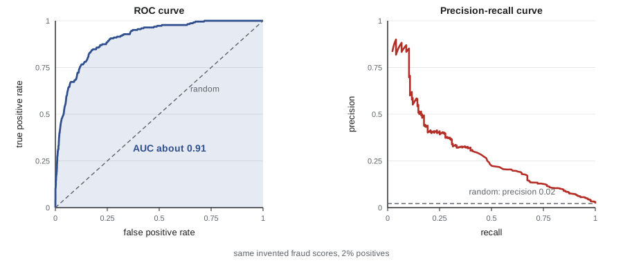
Threshold independence is both the strength and the weakness of AUC. For rare positives, the ROC curve can look excellent while the model's flags are mostly false alarms, because the false positive rate divides by the huge number of negatives. The precision–recall curve, and its summary the average precision, keep attention on the positive class: a random scorer's average precision equals the positive rate, here 2 per cent, so the model's average precision is much more informative about what an investigator will experience. For heavily imbalanced problems, report both.

Calibration

Many applications use predicted probabilities directly: to compute expected costs, to set prices, or to combine evidence. A model is calibrated if, among all cases it assigns probability 0.7, about 70 per cent are positive. Calibration is checked with a reliability diagram, which bins predictions and plots the mean predicted probability against the observed frequency in each bin, and summarized with the Brier score, the mean squared difference between predicted probability and outcome. Logistic regression is usually well calibrated. Naive Bayes, boosted trees and SVM scores usually are not, and modern neural networks tend to be overconfident.

Two standard repairs fit a mapping from scores to probabilities on held-out data. Platt scaling (1999) fits a logistic regression with the model's score, or log odds, as its only input. Isotonic regression fits any monotone step function and is more flexible but needs more data. Both must be fitted on data not used to train the model, or they will learn the model's overconfidence on its own training set.

# Calibration: reliability table and Brier score for an overconfident model, before and after Platt scaling.
import numpy as np
from sklearn.linear_model import LogisticRegression
rng = np.random.default_rng(2)
n = 20_000
true_p = rng.uniform(0.02, 0.98, n)
y = (rng.uniform(size=n) < true_p).astype(int)
logit = np.log(true_p / (1 - true_p))
raw = 1 / (1 + np.exp(-2.5 * logit))                         # an overconfident model: logits stretched 2.5x

def reliability(p, y, bins=5):
    edges = np.linspace(0, 1, bins + 1)
    for lo, hi in zip(edges[:-1], edges[1:]):
        m = (p >= lo) & (p < hi) if hi < 1 else (p >= lo)
        print(f"   predicted {lo:.1f}-{hi:.1f}: mean prediction {p[m].mean():.3f}, observed rate {y[m].mean():.3f}  (n={m.sum()})")

half = n // 2                                                # fit the calibrator on one half, test on the other
platt = LogisticRegression().fit(np.log(raw[:half] / (1 - raw[:half]))[:, None], y[:half])
cal = platt.predict_proba(np.log(raw[half:] / (1 - raw[half:]))[:, None])[:, 1]
for name, p in [("raw model", raw[half:]), ("after Platt scaling", cal)]:
    print(f"{name}: Brier score {np.mean((p - y[half:]) ** 2):.4f}")
    reliability(p, y[half:])

raw model: Brier score 0.1946
   predicted 0.0-0.2: mean prediction 0.051, observed rate 0.188  (n=3581)
   predicted 0.2-0.4: mean prediction 0.294, observed rate 0.413  (n=976)
   predicted 0.4-0.6: mean prediction 0.500, observed rate 0.511  (n=856)
   predicted 0.6-0.8: mean prediction 0.705, observed rate 0.563  (n=1059)
   predicted 0.8-1.0: mean prediction 0.950, observed rate 0.804  (n=3528)
after Platt scaling: Brier score 0.1750
   predicted 0.0-0.2: mean prediction 0.108, observed rate 0.110  (n=1944)
   predicted 0.2-0.4: mean prediction 0.301, observed rate 0.298  (n=1981)
   predicted 0.4-0.6: mean prediction 0.502, observed rate 0.493  (n=2027)
   predicted 0.6-0.8: mean prediction 0.700, observed rate 0.676  (n=2039)
   predicted 0.8-1.0: mean prediction 0.895, observed rate 0.878  (n=2009)

Before calibration, the model's extreme predictions are too extreme: in the top bin it predicts nearly certainty, but the observed rate is lower. After Platt scaling the mean prediction and observed rate agree in every bin and the Brier score falls. Note that recalibration does not change the ranking of cases, so the AUC is unchanged; calibration and discrimination are separate qualities, and a model needs both.

Regression metrics

For regression, the common measures are the mean squared error and its square root (RMSE), in the units of the target; the mean absolute error (MAE), which is less influenced by large errors; and \(R^2 = 1 - \mathrm{MSE}/\mathrm{Var}(y)\), the fraction of variance explained, which is negative for a model worse than predicting the mean. The mean absolute percentage error is popular in forecasting but explodes when targets are near zero. As with classification, choose the metric that reflects the cost of errors in the application, and compare against a naive baseline such as predicting the training mean or, for time series, the last observed value.

Is one model really better?

Suppose model B scores 1.5 points higher than model A on the same test set. Because both were evaluated on the same examples, their errors are correlated, and the right comparison is paired: what matters is how often they disagree, and in whose favour. McNemar's test counts the examples where A is right and B wrong (b) and where A is wrong and B right (c); under the null hypothesis that the models are equally accurate, b and c should be similar, and \((\lvert b - c \rvert - 1)^2 / (b + c)\) has approximately a chi-squared distribution with one degree of freedom.

# Comparing two classifiers on the same test set with McNemar's test.
import numpy as np
from scipy.stats import chi2
rng = np.random.default_rng(9)
m = 1000
correct_a = rng.uniform(size=m) < 0.86                       # model A right on about 86%
correct_b = np.where(rng.uniform(size=m) < 0.8, correct_a, rng.uniform(size=m) < 0.89)
b = np.sum(correct_a & ~correct_b)                            # A right, B wrong
c = np.sum(~correct_a & correct_b)                            # A wrong, B right
stat = (abs(b - c) - 1) ** 2 / (b + c)                        # with continuity correction
print(f"accuracy A {correct_a.mean():.3f}, accuracy B {correct_b.mean():.3f}")
print(f"disagreements: A right/B wrong = {b}, A wrong/B right = {c}")
print(f"McNemar statistic {stat:.2f}, p-value {chi2.sf(stat, df=1):.3f}")
se = np.sqrt(correct_a.mean() * (1 - correct_a.mean()) / m)
print(f"for comparison, the standard error of a single accuracy estimate is {se:.3f}")

accuracy A 0.866, accuracy B 0.875
disagreements: A right/B wrong = 11, A wrong/B right = 20
McNemar statistic 2.06, p-value 0.151
for comparison, the standard error of a single accuracy estimate is 0.011

B is ahead by about one point, but the whole difference rests on 31 disagreements, split 20 to 11, and the p-value of 0.15 says a split this uneven would be unremarkable if the models were equally accurate. A larger test set, or a cross-validated comparison, would be needed to settle the question. With cross-validation, a paired comparison uses the per-fold differences, though the folds' training sets overlap and the naive t-test is somewhat optimistic; Dietterich's 5×2 cross-validation test and the corrected resampled t-test of Nadeau and Bengio address this. When many models or data sets are compared, multiple-comparison corrections apply, as STAT-151 discussed. More important than any test is to avoid the selection effect: if fifty variants were tried, the best is likely to look better than it is, and only a fresh test set can say by how much.

Reporting results

A trustworthy evaluation report states: the data source and population, and how training, validation and test data were split (randomly, by group or by time); the baselines; the metrics, chosen for the application, with uncertainty; how hyperparameters were tuned; and how many configurations were tried. Model cards (Mitchell and colleagues, 2019) and dataset documentation standards, which AI-460 and AI-220 discuss, add intended use, performance across subgroups, and known limitations. Reporting performance separately for relevant subgroups often reveals that an acceptable average hides unacceptable failures for some people.

Worked examples