
ELE-202 · Lesson 5 of 12 · 32 min
Matrix methods and computer-aided circuit analysis
Lesson 4 showed that nodal and mesh analysis turn any linear resistive circuit into a set of simultaneous linear equations. By hand, three or four unknowns are manageable; real circuits have hundreds or millions. Every circuit simulator, from SPICE to the tools used to design integrated circuits and power grids, solves those equations by computer, using the same ideas you already know organized in matrix form. This lesson shows how the matrices are built directly from the circuit, how voltage sources are handled by modified nodal analysis, how to solve the equations with NumPy, and how to use the results to find sensitivities and Thévenin equivalents. It also introduces SPICE and the habits that keep computer results trustworthy.
Nodal analysis as a matrix equation
For a circuit with \(n\) non-reference nodes containing only resistors and independent current sources, nodal analysis gives \(n\) KCL equations that can be written as
where \(\mathbf{v}\) is the vector of unknown node voltages, \(\mathbf{i}\) the vector of source currents injected into each node, and \(\mathbf{G}\) the conductance matrix. \(\mathbf{G}\) can be written down by inspection:
- Diagonal entry \(G_{kk}\): the sum of the conductances connected to node \(k\).
- Off-diagonal entry \(G_{jk}\): minus the sum of the conductances connected directly between nodes \(j\) and \(k\).
- Entry \(i_{k}\): the sum of source currents flowing into node \(k\).
For circuits of resistors and independent sources, \(\mathbf{G}\) is symmetric, and because each resistor touches at most two nodes, it is mostly zeros (sparse) for large circuits.
import numpy as np

# Nodal analysis by hand-built matrices: G v = i
# Circuit: 2 mA source into node 1; 1 kOhm from node 1 to ground; 2 kOhm between nodes 1 and 2;
# 4 kOhm from node 2 to ground; 3 kOhm between nodes 2 and 3; 6 kOhm from node 3 to ground;
# 1 mA source into node 3.
g = lambda r: 1 / r
G = np.array([
    [g(1e3) + g(2e3), -g(2e3),                   0],
    [-g(2e3),          g(2e3) + g(4e3) + g(3e3), -g(3e3)],
    [0,               -g(3e3),                   g(3e3) + g(6e3)],
])
i = np.array([2e-3, 0, 1e-3])
v = np.linalg.solve(G, i)
for k, vk in enumerate(v, start=1):
    print(f"v{k} = {vk:.4f} V")
print("KCL satisfied at every node:", np.allclose(G @ v, i))v1 = 1.9733 V v2 = 1.9200 V v3 = 3.2800 V KCL satisfied at every node: True
The final line checks the answer by substituting it back: \(\mathbf{G}\mathbf{v}\) equals \(\mathbf{i}\), so KCL holds at every node. This kind of check costs one line and catches mistakes in setting up the matrix, which are far more common than errors in solving it.
Element stamps
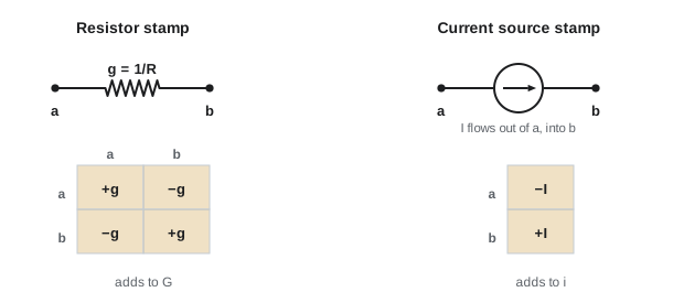
Writing the matrix by inspection is the human view. A program does the same thing element by element. Each resistor of conductance \(g = 1/R\) between nodes \(a\) and \(b\) adds \(+g\) to \(G_{aa}\) and \(G_{bb}\), and \(-g\) to \(G_{ab}\) and \(G_{ba}\). If one end is ground, only the diagonal entry of the other node is changed. Each current source adds to two entries of \(\mathbf{i}\). Adding up the stamps of all elements produces exactly the matrix you would write by inspection. This is why a simulator can accept a circuit in any order: it simply loops over the list of elements.
Modified nodal analysis
Voltage sources do not fit plain nodal analysis, because the current through a voltage source is not determined by its voltage. Lesson 4 handled them with supernodes. Modified nodal analysis (MNA), used by SPICE and nearly every simulator since the 1970s, handles them systematically instead: for each voltage source, it adds the source's current as an extra unknown and the source's voltage relation as an extra equation:
Here \(\mathbf{B}\) has a \(+1\) and a \(-1\) in each column marking the nodes a voltage source connects, \(\mathbf{i}_{V}\) holds the unknown source currents, and \(\mathbf{e}\) the known source voltages. Dependent sources, op amps (Lesson 8), inductors in DC steady state (as zero-volt sources) and many other elements fit the same framework with their own stamps.
import numpy as np

def mna(netlist, n_nodes):
    """Modified nodal analysis. Node 0 is ground. Elements:
    ("R", a, b, ohms), ("I", a, b, amps) flowing from a to b inside the source,
    ("V", a, b, volts) with node a positive."""
    vsrc = [e for e in netlist if e[0] == "V"]
    size = n_nodes + len(vsrc)
    A, z = np.zeros((size, size)), np.zeros(size)
    def add(r, c, val):
        if r > 0 and c > 0:
            A[r - 1, c - 1] += val
    for kind, a, b, val in netlist:
        if kind == "R":
            for r, c, s in [(a, a, 1), (b, b, 1), (a, b, -1), (b, a, -1)]:
                add(r, c, s / val)
        elif kind == "I":
            if a: z[a - 1] -= val
            if b: z[b - 1] += val
    for k, (_, a, b, val) in enumerate(vsrc):
        row = n_nodes + k
        if a: A[row, a - 1] = A[a - 1, row] = 1
        if b: A[row, b - 1] = A[b - 1, row] = -1
        z[row] = val
    x = np.linalg.solve(A, z)
    return x[:n_nodes], x[n_nodes:]

# A 12 V source, a bridge of four resistors and a 1 kOhm load between the bridge midpoints
net = [("V", 1, 0, 12.0),
       ("R", 1, 2, 1000), ("R", 2, 0, 2000),
       ("R", 1, 3, 1500), ("R", 3, 0, 1500),
       ("R", 2, 3, 1000)]
v, i_src = mna(net, 3)
print("Node voltages:", np.round(v, 4))
print(f"Load current (node 2 to 3): {(v[1] - v[2]) / 1000 * 1e3:.3f} mA")
print(f"Source current: {-i_src[0] * 1e3:.3f} mA, power delivered {-i_src[0] * 12:.4f} W")Node voltages: [12. 7.4483 6.6207] Load current (node 2 to 3): 0.828 mA Source current: 8.138 mA, power delivered 0.0977 W
This small function is, in essence, the DC operating-point engine of a circuit simulator. Real simulators add stamps for many more element types, use sparse matrix methods so that circuits with millions of nodes are practical, and wrap the linear solve inside iterative methods (Newton–Raphson) to handle nonlinear devices such as diodes and transistors, and inside time-stepping loops to handle capacitors and inductors (ELE-203).
Worked problem
Setting up MNA by hand
A 10 V source connects node 1 (positive) to ground. A 2 Ω resistor joins nodes 1 and 2, and a 3 Ω resistor joins node 2 to ground. Write the MNA system and solve it.
Show solution
- Unknowns: \(v_{1}\), \(v_{2}\) and the source current \(i_{V}\) (taken as flowing into the positive terminal from node 1).
- KCL at node 1: \(\tfrac{1}{2}v_{1} - \tfrac{1}{2}v_{2} + i_{V} = 0\).
- KCL at node 2: \(-\tfrac{1}{2}v_{1} + (\tfrac{1}{2} + \tfrac{1}{3})v_{2} = 0\).
- Source equation: \(v_{1} = 10\).
- From node 2: \(v_{2} = (1/2)/(5/6) \times 10 = 6\) V. From node 1: \(i_{V} = -(10 - 6)/2 = -2\) A.
Answer: \(v_{1} = 10\) V, \(v_{2} = 6\) V and \(i_{V} = -2\) A: the source delivers 2 A, as expected for 10 V across 5 Ω. The negative sign follows from the reference direction chosen for \(i_{V}\), into the positive terminal, which is the passive sign convention (Lesson 1) and the convention SPICE uses when it reports source currents.
Sensitivity analysis
Once a circuit can be solved in a function call, it can be solved thousands of times. Sensitivity analysis asks how much an output changes when each component changes. The relative sensitivity of output \(y\) to component \(x\) is
A sensitivity of \(+1.2\) means a 1% increase in the component raises the output by about 1.2%. Sensitivities tell the designer which parts need tight tolerances and which can be cheap.
import numpy as np

def load_current(R1, R2, R3, R4, R5, Vs=12.0):
    """Current through R5, connected between the midpoints of a bridge fed by Vs."""
    G = np.array([[1/R1 + 1/R2 + 1/R5, -1/R5],
                  [-1/R5, 1/R3 + 1/R4 + 1/R5]])
    v2, v3 = np.linalg.solve(G, [Vs / R1, Vs / R3])
    return (v2 - v3) / R5

nominal = dict(R1=1000, R2=2000, R3=1500, R4=1500, R5=1000)
i0 = load_current(**nominal)
print(f"Nominal load current: {i0 * 1e3:.4f} mA")
print("Relative sensitivity (% change in current per 1% change in each resistor):")
for name in nominal:
    bumped = dict(nominal, **{name: nominal[name] * 1.01})
    s = (load_current(**bumped) - i0) / i0 / 0.01
print(f" {name}: {s:+.2f}")Nominal load current: 0.8276 mA Relative sensitivity (% change in current per 1% change in each resistor): R1: -1.51 R2: +1.23 R3: +1.34 R4: -1.64 R5: -0.41
The bridge's load current is more sensitive to the four bridge arms (magnitudes 1.2 to 1.6) than to the load resistor itself (0.41). That is because the current depends on a small difference between two divider voltages: a 1% change in an arm changes that difference by more than 1%. Bridge-type circuits, differential amplifiers and anything else that subtracts nearly equal quantities magnify component errors, so their critical parts must be precise or matched.
Worked problem
From sensitivities to an error budget
Using the sensitivities above and resistors of ±0.5% tolerance, estimate the worst-case and the root-sum-square (statistical) variation of the load current.
Show solution
- Worst case: \(0.5\% \times (1.51 + 1.23 + 1.34 + 1.64 + 0.41) = 0.5\% \times 6.13 = 3.1\%\).
- Root-sum-square: \(0.5\% \times \sqrt{1.51^{2} + 1.23^{2} + 1.34^{2} + 1.64^{2} + 0.41^{2}} = 0.5\% \times \sqrt{8.45} = 1.5\%\).
Answer: Up to about ±3.1% if every resistor is at its worst limit at once, and about ±1.5% as a typical spread if their errors are independent. The first guarantees the design; the second predicts production. Lesson 12 checks such estimates with Monte Carlo simulation.
Thévenin equivalents by computer
Lesson 6 finds Thévenin equivalents by hand. A computer finds them by two solutions of the same circuit: the open-circuit voltage gives \(V_{th}\), and the short-circuit current gives \(I_{N}\), so that \(R_{th} = V_{th}/I_{N}\). In code, "open" and "short" can be approximated by very large and very small load resistances, as long as they are far beyond any resistance in the circuit.
import numpy as np

def node_voltages(RL, Vs=12.0, R1=1000, R2=2000, R3=1500, R4=1500):
    G = np.array([[1/R1 + 1/R2 + 1/RL, -1/RL],
                  [-1/RL, 1/R3 + 1/R4 + 1/RL]])
    return np.linalg.solve(G, [Vs / R1, Vs / R3])

# Thevenin equivalent seen by the load, found numerically
v_open = np.subtract(*node_voltages(1e12))            # load removed (open circuit)
v_short_i = np.subtract(*node_voltages(1e-6)) / 1e-6  # load replaced by a near short
Rth = v_open / v_short_i
print(f"Vth = {v_open:.4f} V, Rth = {Rth:.1f} ohm")

RL = np.linspace(100, 3000, 2901)
P = np.array([np.subtract(*node_voltages(r))**2 / r for r in RL])
best = RL[P.argmax()]
print(f"Maximum load power {P.max() * 1e3:.3f} mW at RL = {best:.0f} ohm")
print(f"Theory: Vth^2 / (4 Rth) = {v_open**2 / (4 * Rth) * 1e3:.3f} mW")Vth = 2.0000 V, Rth = 1416.7 ohm Maximum load power 0.706 mW at RL = 1417 ohm Theory: Vth^2 / (4 Rth) = 0.706 mW
The computed \(R_{th} = 1416.7\) Ω matches the hand result \(1\,\text{k}\Omega \parallel 2\,\text{k}\Omega + 1.5\,\text{k}\Omega \parallel 1.5\,\text{k}\Omega = 666.7 + 750\) Ω, and the sweep confirms that load power peaks when \(R_{L} = R_{th}\), at \(V_{th}^{2}/4R_{th}\).
SPICE
SPICE (Simulation Program with Integrated Circuit Emphasis) was developed at the University of California, Berkeley, in the early 1970s and is the ancestor of nearly every analog circuit simulator: commercial tools such as Cadence Spectre and PSpice, free ones such as LTspice and ngspice, and the simulators built into PCB design packages. A SPICE circuit is described by a netlist, one line per element, naming the element, the nodes it connects (node 0 is ground) and its value.
| Netlist line | Meaning |
|---|---|
| V1 1 0 DC 12 | 12 V source, node 1 positive, node 0 (ground) negative |
| R1 1 2 1k | 1 kΩ between nodes 1 and 2 |
| R2 2 0 2k | 2 kΩ from node 2 to ground |
| R3 1 3 1.5k | 1.5 kΩ between nodes 1 and 3 |
| R4 3 0 1.5k | 1.5 kΩ from node 3 to ground |
| RL 2 3 1k | 1 kΩ load between nodes 2 and 3 |
| .op | Compute the DC operating point |
| .dc V1 0 12 0.5 | Sweep V1 from 0 to 12 V in 0.5 V steps |
| .end | End of netlist |
Beyond the DC operating point (.op) and DC sweeps (.dc), SPICE performs transient analysis (.tran), AC frequency response (.ac), noise, sensitivity, Monte Carlo and worst-case analyses, using models of real diodes, transistors, op amps and other parts supplied by manufacturers.
Trusting computer results
Simulators solve exactly the circuit you describe, which may not be the one you meant. Good habits:
- Estimate first. Know roughly what answer to expect before running anything, from a quick hand analysis or a simplified circuit.
- Check conservation. Total power delivered by sources should equal total power absorbed, and KCL should hold at every node.
- Watch for floating nodes. A node with no DC path to ground makes the matrix singular, and the simulator will report an error or invent a result; capacitors and current sources in series commonly cause this.
- Beware ill-conditioning. Circuits mixing very large and very small resistances (such as 1 mΩ shunts and 10 MΩ dividers) produce matrices whose solutions are sensitive to rounding. Simulators use tolerances and scaling; unexpected results in such circuits deserve suspicion.
- Remember that models are approximations. A simulated op amp or transistor is only as good as its model, and a resistor model usually lacks tolerance, temperature effects and parasitic inductance unless you add them.
Worked problem
A singular matrix
A student simulates two 1 kΩ resistors in series with a capacitor, driven by a DC current source, and the DC analysis fails with "singular matrix". Why?
Show solution
- In DC analysis, a capacitor is an open circuit (Lesson 10).
- The current source then drives current into a node with no DC path to ground: KCL at that node cannot be satisfied for any voltage.
- Mathematically, the row of the conductance matrix for that node, or a group of nodes, is all zeros or linearly dependent.
Answer: The circuit has no DC solution: an ideal current source charging an ideal capacitor drives its voltage to infinity. The fix is to describe the circuit that was really intended, for example by adding a large resistor across the capacitor to model its leakage, or by running a transient analysis instead.
Common mistakes
MistakeWriting off-diagonal conductance entries as positive.
InsteadOff-diagonal entries are minus the conductance between the two nodes.
MistakeForgetting that voltage sources need extra unknowns in nodal form.
InsteadUse supernodes by hand, or MNA with source currents as unknowns.
MistakeTrusting a simulation result without an estimate or check.
InsteadEstimate first, then check KCL and power balance.
MistakeLeaving a node without a DC path to ground.
InsteadMake sure every node has a DC path, or model leakage explicitly.
MistakeUsing worst-case sums when a statistical estimate is wanted, or the reverse.
InsteadUse worst case to guarantee limits and root-sum-square or Monte Carlo to predict yield.
Summary and key terms
- Nodal analysis of resistive circuits is the matrix equation Gv = i, with G written by inspection or built from stamps.
- Modified nodal analysis adds voltage-source currents as unknowns, and is the basis of SPICE.
- numpy.linalg.solve solves the system; substitute back to check KCL.
- Relative sensitivities identify the components that most affect an output.
- Thévenin equivalents follow from open-circuit and short-circuit solutions.
- SPICE netlists describe circuits line by line for many kinds of analysis.
- Estimate first, check conservation, avoid floating nodes and remember model limits.
- Conductance matrix
- The matrix G relating node voltages to injected currents.
- Stamp
- The pattern of matrix entries an element contributes.
- Modified nodal analysis
- Nodal analysis extended with voltage-source currents as unknowns.
- Sparse matrix
- A matrix in which most entries are zero.
- Relative sensitivity
- The percentage change in an output per percentage change in a component.
- Root-sum-square
- Combining independent errors as the square root of the sum of squares.
- SPICE
- The family of circuit simulators descended from Berkeley's 1970s program.
- Netlist
- A text description of a circuit listing elements, nodes and values.
- Singular matrix
- A matrix with no inverse, indicating no unique solution.
- Ill-conditioning
- Sensitivity of a solution to small errors in the matrix.
Practice problems
Work each problem on paper first, then reveal the answer to check.
A node connects to 2 kΩ, 4 kΩ and 4 kΩ resistors. Its diagonal entry in G?
Show answer
1 mS (0.5 + 0.25 + 0.25 mS).
A 5 kΩ resistor joins nodes 2 and 3. Its contribution to G₂₃?
Show answer
−0.2 mS.
Is G symmetric for circuits of resistors and independent sources?
Show answer
Yes.
How many unknowns does MNA have for 6 nodes and 2 voltage sources?
Show answer
8.
5 V source to node 1; 1 Ω from node 1 to node 2; 4 Ω node 2 to ground. v₂?
Show answer
4 V.
A 1% increase in R raises the output by 0.3%. Relative sensitivity?
Show answer
+0.3.
Sensitivities 1, 1, 2 with ±1% parts. Worst-case and RSS variation?
Show answer
4% and √6 ≈ 2.4%.
Open-circuit voltage 6 V, short-circuit current 3 mA. Rth?
Show answer
2 kΩ.
Write a SPICE line for a 470 Ω resistor between nodes 4 and 0.
Show answer
R5 4 0 470 (any unique name starting with R).
Why does a DC analysis fail for a current source feeding only a capacitor?
Show answer
The node has no DC path to ground, so the matrix is singular.
Lesson quiz · 5 questions
Score 60% or more to complete this lesson.
Create a free account to save your progress, take quizzes and earn a certificate.