Sequences, series and Taylor polynomials

Your calculator does not store a table of sines. When you press sin(0.3), it adds up a few terms of a polynomial that matches the sine function extremely well near zero. The same idea runs through engineering: the small-angle approximation, linearized models in control systems, simplified formulas for cable sag and pendulum periods, and the Fourier series that break signals into frequencies. All of them replace a complicated function with an infinite sum of simple terms, then keep only the few that matter.

This lesson builds that toolkit. It starts with sequences and infinite series, develops tests for whether a series adds up to a finite number, and ends with Taylor polynomials: how to build them, how accurate they are, and how engineers use them every day.

Sequences

A sequence is an ordered list of numbers \(a_1, a_2, a_3, \ldots\), usually given by a formula for the \(n\)th term. The sequence converges to \(L\) if its terms get as close to \(L\) as you like for large \(n\): \(\lim_{n \to \infty} a_n = L\). Otherwise it diverges.

The limit techniques from Calculus I all apply, with \(n\) in place of \(x\).

• \(a_n = \dfrac{3n + 1}{n + 4} \to 3\): divide top and bottom by \(n\).
• \(a_n = r^n \to 0\) when \(|r| < 1\), and grows without bound when \(|r| > 1\).
• \(a_n = (-1)^n\) diverges: it bounces between −1 and 1 and never settles.
• \(a_n = \left(1 + \dfrac1n\right)^n \to e\). The terms are 2, 2.594, 2.705 and 2.717 for \(n\) = 1, 10, 100 and 1000. This is how \(e\) arises in compound interest and continuous growth.

Sequences describe anything measured in steps: the state of a system at each time step of a simulation, successive estimates from Newton's method, the balance in an account each month, or the remaining strength of a part after each load cycle.

Series and partial sums

A series adds up the terms of a sequence: \(\sum_{n=1}^{\infty} a_n = a_1 + a_2 + a_3 + \cdots\). An infinite sum is defined through its partial sums \(S_N = a_1 + \cdots + a_N\). If the partial sums converge to a number \(S\), the series converges and its sum is \(S\).

Geometric series

The most important series multiplies each term by a fixed ratio \(r\):

Why: the partial sum is \(S_N = a\dfrac{1 - r^{N+1}}{1 - r}\) (multiply \(S_N\) by \(r\) and subtract to see this). When \(|r| < 1\), \(r^{N+1} \to 0\). When \(|r| \ge 1\) the series diverges.

Repeating decimals

Geometric series also explain why \(0.999\ldots = 1\): it is \(0.9 + 0.09 + 0.009 + \cdots = \dfrac{0.9}{1 - 0.1} = 1\).

Testing for convergence

Most series cannot be summed exactly, but we still need to know whether they converge. Several tests answer that question.

The divergence test

If the terms do not approach zero, the series must diverge. For example, \(\sum \dfrac{n}{n + 1}\) diverges because its terms approach 1. The converse is false: terms going to zero does not guarantee convergence.

The harmonic series

The famous counterexample is the harmonic series:

Group the terms: \(\tfrac13 + \tfrac14 > \tfrac12\), \(\tfrac15 + \cdots + \tfrac18 > \tfrac12\), and so on. Infinitely many groups each exceed \(\tfrac12\), so the sum grows without bound. It grows extremely slowly, though: the first thousand terms add up to only about 7.49, and the first million to about 14.39.

The integral test and p-series

If \(f(x)\) is positive and decreasing, the series \(\sum f(n)\) and the integral \(\int_1^\infty f(x)\,dx\) either both converge or both diverge. The terms of the series are rectangles under (or over) the curve. Combined with the p-test from Lesson 4:

So \(\sum 1/n^2\) converges. Its exact sum, found by Euler, is \(\pi^2/6 \approx 1.6449\).

The ratio test

For series with factorials or powers, compare each term with the next:

If \(L < 1\) the series converges; if \(L > 1\) it diverges; if \(L = 1\) the test gives no answer. The ratio test treats a series as "eventually like a geometric series with ratio \(L\)."

Alternating series

A series whose signs alternate converges if its terms shrink steadily to zero in size. Better still, the error from stopping after \(N\) terms is no bigger than the first term you left out. This makes alternating series very convenient for calculation, because you know exactly how accurate your answer is.

Power series

A power series is an infinite polynomial: \(\sum_{n=0}^{\infty} c_n x^n = c_0 + c_1x + c_2x^2 + \cdots\). Whether it converges depends on \(x\). The ratio test shows that every power series converges for \(|x| < R\) and diverges for \(|x| > R\), for some radius of convergence \(R\) (which can be 0 or ∞).

• The geometric series \(\sum x^n = \dfrac{1}{1 - x}\) has \(R = 1\).
• \(\sum \dfrac{x^n}{n!}\) has \(R = \infty\): the factorial eventually crushes any power.

Inside the radius, power series behave like polynomials. You can differentiate and integrate them term by term, which is what makes them so useful.

Taylor series

Suppose you want a polynomial that matches a function \(f\) near \(x = a\) as closely as possible. Matching the value, the slope, the curvature and every higher derivative at \(a\) gives the Taylor series:

Around \(a = 0\) it is called a Maclaurin series. Stopping after the \((x - a)^n\) term gives the Taylor polynomial of degree \(n\), written \(T_n(x)\). The first two terms are the tangent-line approximation from Calculus I.

The series you will use most:

• \(e^{x} = 1 + x + \dfrac{x^2}{2!} + \dfrac{x^3}{3!} + \cdots\) (all \(x\))
• \(\sin x = x - \dfrac{x^3}{3!} + \dfrac{x^5}{5!} - \cdots\) (all \(x\))
• \(\cos x = 1 - \dfrac{x^2}{2!} + \dfrac{x^4}{4!} - \cdots\) (all \(x\))
• \(\ln(1 + x) = x - \dfrac{x^2}{2} + \dfrac{x^3}{3} - \cdots\) (\(-1 < x \le 1\))
• \((1 + x)^k = 1 + kx + \dfrac{k(k-1)}{2!}x^2 + \cdots\) (binomial series, \(|x| < 1\))

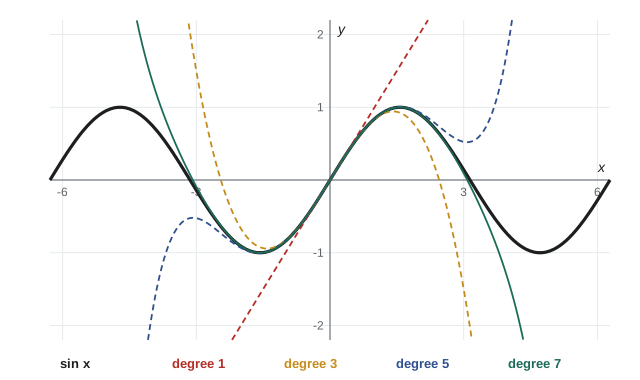
New series can be built from known ones by substitution, multiplication, differentiation or integration, without computing any derivatives. Replacing \(x\) with \(-x^2\) in the exponential series gives \(e^{-x^2} = 1 - x^2 + \dfrac{x^4}{2!} - \cdots\), which can then be integrated term by term. That is how the bell-curve integral from Lesson 1, which has no elementary antiderivative, is computed to any accuracy.

How accurate is a Taylor polynomial?

Taylor's theorem gives the error. If you approximate \(f\) by \(T_n\), the remainder is

for some \(c\) between \(a\) and \(x\). You do not know \(c\) exactly, but you can bound the error by using the largest possible value of \(|f^{(n+1)}|\) on the interval. Two things make the error small: being close to \(a\) (the factor \((x - a)^{n+1}\)), and using more terms (the factorial in the denominator).

Engineering approximations

Taylor polynomials are behind many simplified formulas that engineers use without thinking about where they came from.

Small angles

For small \(\theta\) in radians, \(\sin\theta \approx \theta\), \(\tan\theta \approx \theta\) and \(\cos\theta \approx 1 - \tfrac12\theta^2\). These keep the first nonzero term of each series. At 10° (0.1745 rad), \(\sin\theta\) is 0.1736, an error of 0.5%.

The binomial approximation

For small \(x\), \((1 + x)^k \approx 1 + kx\). It turns awkward expressions into linear ones.

• \(\sqrt{1.1} = (1 + 0.1)^{1/2} \approx 1 + 0.05 = 1.05\). (True: 1.0488. Adding the next term, \(-\tfrac18(0.1)^2\), gives 1.04875.)
• Thermal expansion: a part that grows by a fraction \(\alpha\Delta T\) in each dimension changes volume by \((1 + \alpha\Delta T)^3 \approx 1 + 3\alpha\Delta T\). The volume coefficient is three times the linear one.

Fourier series

Taylor series build functions from powers of \(x\). Fourier series build periodic functions from sines and cosines. Any repeating signal (a square wave from a digital circuit, the vibration of an engine, the current drawn by a rectifier) can be written as a sum of harmonics at whole-number multiples of its base frequency. A square wave of height 1 is

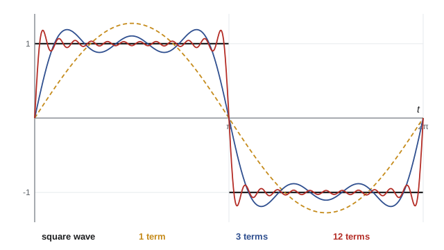
This is how engineers find which frequencies a signal contains: the basis of filters, audio processing, vibration analysis and power-quality measurement. You will study Fourier series and transforms in Signals and Systems.