
PHOT-420 · Lesson 2 of 12 · 32 min
The image signal processor: demosaicing, white balance and noise
Before any clever multi-frame trick or neural network can run, raw sensor numbers must be cleaned, coloured and made linear. These early stages are handled mostly by the image signal processor (ISP), and their quality sets a ceiling on everything that follows. PHOT-201 introduced the Bayer pattern and the idea of demosaicing; this lesson looks inside the algorithms. You will model sensor noise mathematically, run a bilinear demosaicing algorithm on a synthetic image and measure its errors, estimate white balance automatically with two classic methods, and see how a colour correction matrix maps sensor colours to a standard colour space. These are the same building blocks phone and camera engineers tune, and understanding them explains many artefacts photographers see.
The early raw stages
A raw readout is not yet a clean measurement of light. The ISP applies several corrections in order.
- Black level subtraction: even with no light, each pixel reads a small offset value, often 64 or 256 on a 10- or 12-bit scale. This pedestal is subtracted so that zero light reads zero.
- Defective pixel correction: a few pixels are permanently stuck bright (hot) or dark (dead). The ISP keeps a map of them and replaces each with an estimate from neighbours of the same colour.
- Lens shading correction: small lenses deliver less light to the corners than the centre (vignetting) and can shift colour toward the edges. A per-channel gain map, calibrated at the factory for each module, flattens this.
- Linearization: the sensor response is made proportional to light, correcting any nonlinearity near saturation.
- Clipping detection: pixels at or near the saturation value are flagged, because their true value is unknown and later stages, such as HDR merging, must treat them specially.
These steps sound mundane, but errors in them cause familiar problems: coloured corners in phone photos of blank walls come from imperfect lens shading correction; magenta highlights come from mishandled clipping in one channel; a faint pattern in deep shadows can come from an inaccurate black level.
Modelling sensor noise
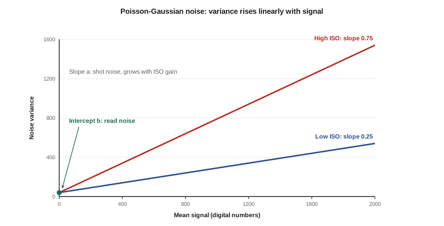
Noise in a raw pixel has two main parts. Shot noise depends on the signal: its variance equals the number of photoelectrons. Read noise comes from the electronics and is roughly constant regardless of signal. Engineers combine them in a Poisson-Gaussian model, in which the variance of a pixel value \( x \) is a linear function of its mean:
Here \( a \) depends on the sensor gain (ISO setting) and \( b \) on read noise. The model is calibrated for each sensor and ISO by photographing flat grey targets and plotting variance against mean. Denoising algorithms, burst merging and HDR all use this noise model to decide how much to trust each pixel. A pixel in a bright area has high absolute noise but high SNR; a pixel in deep shadow has low absolute noise but low SNR because read noise dominates.
Worked problem
Using the noise model
A sensor at a given ISO has \( a = 0.5 \) and \( b = 4 \) (in squared digital numbers). Find the standard deviation and SNR for mean values of 20 and 2,000.
Show solution
- At 20: \( \sigma^2 = 0.5 \times 20 + 4 = 14 \), so \( \sigma \approx 3.74 \) and SNR \( \approx 20/3.74 \approx 5.3 \).
- At 2,000: \( \sigma^2 = 0.5 \times 2000 + 4 = 1004 \), so \( \sigma \approx 31.7 \) and SNR \( \approx 63 \).
- Read noise is a large share of the variance at 20 (4 of 14) but negligible at 2,000.
Answer: SNR is about 5 in the shadow and 63 in the bright tone; shadows are limited partly by read noise, which merging many short frames does not reduce as efficiently as one long frame.
That last point matters for burst photography. Each frame contributes its own read noise, so merging \( n \) short frames has \( n \) times the read noise variance of one long frame with the same total exposure. Modern sensors have very low read noise, which is part of why burst methods work so well; lesson 6 returns to this trade-off in night modes.
Demosaicing algorithms
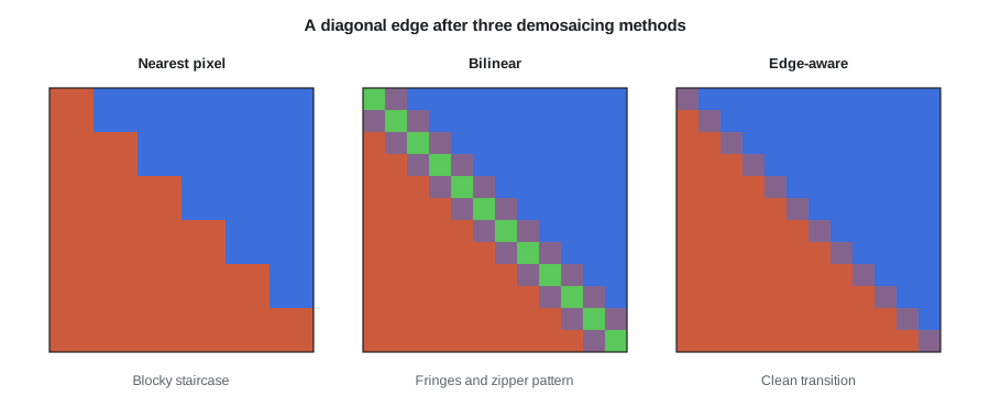
A Bayer colour filter array records red at one pixel in four, blue at one in four and green at two in four. Demosaicing estimates the two missing colours at every pixel. The simplest method, bilinear interpolation, averages the nearest neighbours of each colour. At a red pixel, for example, the missing green is the average of the four green neighbours above, below, left and right, and the missing blue is the average of the four diagonal blue neighbours. Bilinear interpolation is fast and works well in smooth areas, but at sharp edges it averages across the edge, producing colour fringes and zipper artefacts, a jagged alternating pattern along edges.
Better algorithms are edge-aware. They estimate the direction of local edges, horizontal or vertical, and interpolate along rather than across them. Others exploit the fact that colour differences (red minus green, blue minus green) vary more smoothly than colours themselves, so they interpolate green first at full resolution and then interpolate the colour differences. Well-known methods include adaptive homogeneity-directed (AHD) demosaicing and the many variants in raw converters. Since about 2016, learned demosaicing using convolutional neural networks has outperformed hand-designed methods on benchmarks, and joint demosaicing and denoising networks treat both problems together, because noise and missing samples interact.
import numpy as np
rng = np.random.default_rng(420)
h, w = 32, 32
img = np.zeros((h, w, 3))
img[:, :16] = [0.8, 0.3, 0.2]          # warm left half
img[:, 16:] = [0.2, 0.4, 0.9]          # cool right half: a sharp vertical edge
img += rng.normal(0, 0.005, img.shape)  # a little texture
# RGGB Bayer mosaic: keep one channel per pixel
mask = np.zeros((h, w, 3), bool)
mask[0::2, 0::2, 0] = True              # R
mask[0::2, 1::2, 1] = True              # G
mask[1::2, 0::2, 1] = True              # G
mask[1::2, 1::2, 2] = True              # B
mosaic = np.where(mask, img, 0.0)
def conv3(x, k):
    p = np.pad(x, 1, mode="reflect")
    return sum(k[i, j] * p[i:i + h, j:j + w] for i in range(3) for j in range(3))
k_g = np.array([[0, 1, 0], [1, 4, 1], [0, 1, 0]]) / 4
k_rb = np.array([[1, 2, 1], [2, 4, 2], [1, 2, 1]]) / 4
out = np.stack([conv3(mosaic[..., 0], k_rb), conv3(mosaic[..., 1], k_g), conv3(mosaic[..., 2], k_rb)], -1)
err = np.abs(out - img).mean(axis=2)
print(f"mean error away from the edge: {err[:, 2:12].mean():.4f}")
print(f"mean error in the 4 columns at the edge: {err[:, 14:18].mean():.4f}")
print(f"edge error is {err[:, 14:18].mean() / err[:, 2:12].mean():.0f} times larger")mean error away from the edge: 0.0032 mean error in the 4 columns at the edge: 0.0581 edge error is 18 times larger
The output shows the core weakness of bilinear demosaicing: error near the edge is many times larger than in flat areas, and because each channel is interpolated from different positions, the errors differ by channel and appear as colour fringes. Edge-aware and learned methods attack exactly this region.
Aliasing, moiré and false colour
Fine repeating patterns, such as fabric weaves, screens and distant brickwork, can contain detail finer than the colour filter array samples. The result is aliasing: false patterns and false colours that were not in the scene. Many dedicated cameras have removed the optical low-pass filter that used to blur detail slightly to prevent this, relying on high pixel counts and software. Phones use very small pixels and typically bin pixels in quad-Bayer arrangements (groups of four same-colour pixels), which changes the sampling and requires special remosaicing algorithms when full resolution is wanted. Learned demosaicing reduces moiré considerably but cannot recover detail that was never sampled; it can only make a plausible guess. PHOT-201 covers pixel-shift modes, which avoid demosaicing by capturing each colour at each location.
| Approach | Speed | Quality at edges | Typical use |
|---|---|---|---|
| Nearest neighbour | Very fast | Poor, blocky | Previews only |
| Bilinear | Fast | Colour fringes, zippering | Simple pipelines, teaching |
| Edge-directed and colour-difference | Moderate | Good | ISPs and many raw converters |
| Learned (neural network) | Slower, needs NPU or GPU | Best on benchmarks | Phones, AI-enhanced raw converters |
| Joint demosaic and denoise | Slower | Best in low light | Burst pipelines, night modes |
White balance algorithms
The colour of light varies widely, from warm tungsten to cool shade, and the eye adapts to it. A camera must estimate the illuminant and apply per-channel gains so that neutral surfaces appear neutral. This is automatic white balance (AWB). Two classic assumptions are easy to compute. The grey world assumption says that the average colour of a scene is neutral grey, so the gains should equalize the channel means. The white patch (or max-RGB) assumption says that the brightest surface is white, so the gains should equalize the channel maxima. Both fail predictably: grey world fails when a scene is dominated by one colour, such as a forest or a red wall, and white patch fails when there is no white surface or when the brightest pixels are clipped or coloured light sources.
import numpy as np
rng = np.random.default_rng(420)
n = 5000
reflect = rng.uniform(0.05, 0.9, (n, 3))      # random surfaces
reflect[:50] = 0.95                            # a few white surfaces
light = np.array([1.0, 0.8, 0.55])             # warm illuminant (relative R, G, B)
seen = reflect * light
def gains_avg(x): m = x.mean(axis=0); return m[1] / m
def gains_max(x): m = np.percentile(x, 99.5, axis=0); return m[1] / m
true = light[1] / light
for name, g in [("average", gains_avg(seen)), ("max-RGB", gains_max(seen))]:
    print(f"{name:8s} gains R {g[0]:.2f} G {g[1]:.2f} B {g[2]:.2f}  error {np.abs(g - true).max():.3f}")
print(f"true gains R {true[0]:.2f} G {true[1]:.2f} B {true[2]:.2f}")
# a scene dominated by green foliage breaks the average method
fol = reflect * np.array([0.4, 1.0, 0.4])
g = gains_avg(fol * light)
print(f"foliage scene, average-method gains R {g[0]:.2f} B {g[2]:.2f} (true R {true[0]:.2f} B {true[2]:.2f})")average gains R 0.78 G 1.00 B 1.45 error 0.017 max-RGB gains R 0.80 G 1.00 B 1.45 error 0.000 true gains R 0.80 G 1.00 B 1.45 foliage scene, average-method gains R 1.96 B 3.62 (true R 0.80 B 1.45)
In the program, "average" is the grey world method and "max-RGB" is the white patch method. Both recover the warm illuminant well on a varied scene, but grey world badly overcorrects the foliage scene, pushing it toward magenta. Modern phones use learned AWB: a neural network trained on thousands of scenes with known illuminants, often combined with face detection, an ambient light sensor and scene recognition. Google's approach, for example, has been described as a learning-based method trained on large labelled datasets. Even so, mixed lighting, such as a window and tungsten lamp in one room, has no single correct answer, and some pipelines now apply different white balance to different regions.
The colour correction matrix
After white balance, sensor colours still do not match a standard colour space, because the sensor's red, green and blue filters have different spectral responses from the human eye's cones and from the primaries of sRGB or Display P3. A colour correction matrix (CCM), a 3 by 3 matrix calibrated for each sensor, maps white-balanced camera RGB to linear standard RGB:
Each row usually sums to 1 so that neutral greys stay neutral. Large off-diagonal values, typically negative, increase saturation to compensate for overlapping filter responses, but they also amplify noise, because subtracting noisy channels from each other adds their variances. This is one reason low-light colour looks blotchy: the CCM amplifies chroma noise. Raw converters often use two CCMs calibrated under different illuminants and interpolate between them according to the estimated white balance. Professional colour management, covered in PHOT-202, starts from this point.
Worked problem
Applying a colour correction matrix
A white-balanced camera pixel reads \( (0.50, 0.40, 0.30) \). The first row of the CCM is \( (1.6, -0.4, -0.2) \). Find the output red value and check that the row preserves neutrals.
Show solution
- Output red \( = 1.6 \times 0.50 - 0.4 \times 0.40 - 0.2 \times 0.30 = 0.80 - 0.16 - 0.06 = 0.58 \).
- Row sum \( = 1.6 - 0.4 - 0.2 = 1.0 \), so a neutral input \( (k, k, k) \) gives red \( = k \).
Answer: Output red is 0.58, slightly more saturated than the input; the row sums to one, so greys stay grey.
Worked problem
Noise amplification by the matrix
Each input channel has independent noise standard deviation 0.01. Estimate the noise standard deviation of the output red channel using the row \( (1.6, -0.4, -0.2) \).
Show solution
- Variances add with squared coefficients: \( (1.6^2 + 0.4^2 + 0.2^2) \times 0.01^2 \).
- \( 2.56 + 0.16 + 0.04 = 2.76 \), so the variance is \( 2.76 \times 10^{-4} \).
- Standard deviation \( = 0.01 \times \sqrt{2.76} \approx 0.0166 \).
Answer: Noise rises by about two-thirds in the red channel, which is why strong colour correction worsens visible noise in low light.
Tuning, artefacts and what photographers see
ISP tuning is a craft. Image quality engineers adjust dozens of parameters, from demosaicing thresholds to noise reduction strength at each ISO, and test them on standard charts and thousands of real scenes. Common artefacts trace back to these stages: maze-like patterns in fine texture come from demosaicing; colour shifts in corners come from lens shading; waxy skin comes from noise reduction applied before or during demosaicing; colour casts in mixed light come from AWB. Raw converters let you redo some stages with different algorithms, which is why converting the same raw file in two programs can give visibly different detail. When you evaluate a phone or camera for professional use, test fine fabric, foliage, mixed light and deep shadow, because these are where ISP choices show.
| Artefact | What you see | Usual source |
|---|---|---|
| Zippering and colour fringes | Jagged coloured edges | Demosaicing |
| Moiré and false colour | Rainbow patterns in fabric or screens | Aliasing before demosaicing |
| Colour shading | Corners tinted green or magenta | Lens shading correction |
| Magenta highlights | Pink tint in clipped skies or lamps | Clipping handled per channel |
| Chroma blotches | Coloured mottling in shadows | Noise amplified by the colour matrix |
| Waxy texture | Smooth, plastic skin or foliage | Strong noise reduction |
Common mistakes
MistakeTreating raw values as already proportional to light
InsteadRemember black level subtraction and linearization must happen before any maths on raw values.
MistakeAssuming bilinear demosaicing is good enough everywhere
InsteadExpect fringes and zippering at edges; use edge-aware or learned methods for critical detail.
MistakeTrusting grey-world white balance in scenes dominated by one colour
InsteadCheck AWB on forests, walls and sunsets, and set white balance manually or with a target when it matters.
MistakeIgnoring that colour correction amplifies noise
InsteadExpect more chroma noise in low light and reduce saturation or apply chroma noise reduction.
MistakeBlaming the lens for coloured corners
InsteadCheck lens shading correction, which is a calibration step in the pipeline.
Summary and key terms
- The ISP subtracts black level, corrects defective pixels and lens shading, linearizes and flags clipping before other processing.
- Sensor noise follows a Poisson-Gaussian model with variance \( a\mu + b \), calibrated per sensor and ISO.
- Bilinear demosaicing is simple but produces fringes and zippering at edges; edge-aware and learned methods do better.
- Aliasing creates moiré and false colour that demosaicing can hide but not truly recover.
- Grey-world and white-patch AWB are simple but fail in predictable scenes; phones now use learned AWB.
- A colour correction matrix maps camera RGB to standard RGB, preserving neutrals but amplifying noise.
- Many visible artefacts can be traced to specific ISP stages.
- Black level
- The pixel value recorded with no light, subtracted to make values proportional to light.
- Lens shading correction
- Per-channel gain maps that correct vignetting and colour shifts toward the frame edges.
- Poisson-Gaussian noise model
- A model in which noise variance equals a slope times the mean signal plus a constant read-noise term.
- Read noise
- Noise added by the sensor electronics, roughly independent of signal.
- Bilinear demosaicing
- Estimating missing colours by averaging nearest neighbours of the same colour.
- Zippering
- A jagged alternating artefact along edges caused by poor demosaicing.
- Grey world assumption
- The assumption that a scene's average colour is neutral, used to estimate white balance.
- White patch assumption
- The assumption that the brightest surface in a scene is white.
- Colour correction matrix (CCM)
- A 3 by 3 matrix converting camera RGB to a standard colour space.
- Quad-Bayer
- A sensor layout with groups of four same-colour pixels, often binned for low light.
Practice problems
Work each problem on paper first, then reveal the answer to check.
Why must black level be subtracted before white balance gains are applied?
Show answer
Otherwise the offset is multiplied by different gains per channel, creating colour casts in shadows.
With \( a = 1 \) and \( b = 9 \), what is the noise standard deviation at a mean of 16?
Show answer
\( \sqrt{16 + 9} = 5 \).
Why does merging many short frames carry more read noise than one long exposure?
Show answer
Each frame adds its own read noise, so total read noise variance grows with the number of frames.
Describe how bilinear interpolation estimates green at a red pixel.
Show answer
It averages the four green neighbours above, below, left and right.
Why do edge-aware methods reduce fringes?
Show answer
They interpolate along edges rather than across them, avoiding averaging dissimilar colours.
When does grey-world white balance fail?
Show answer
When a scene is dominated by one colour, such as foliage or a coloured wall.
A CCM row is \( (1.5, -0.3, -0.2) \). Does it preserve neutrals?
Show answer
Yes, it sums to 1.0.
Compute output green for input \( (0.4, 0.5, 0.2) \) with row \( (-0.2, 1.4, -0.2) \).
Show answer
\( -0.08 + 0.70 - 0.04 = 0.58 \).
Name the likely source of rainbow patterns on a photographed computer screen.
Show answer
Aliasing (moiré) from the colour filter array sampling.
What scenes would you test to evaluate a phone's ISP?
Show answer
Fine fabric or foliage, mixed lighting, deep shadows and clipped highlights.
Lesson quiz · 5 questions
Score 60% or more to complete this lesson.
Create a free account to save your progress, take quizzes and earn a certificate.