
PHOT-420 · Lesson 9 of 12 · 30 min
Generative AI fundamentals for imaging
Everything so far in this course has started from light captured by a sensor. Generative AI can produce a photorealistic image from nothing but a sentence, extend a frame beyond its edges, replace a sky or remove a person seamlessly. For photographers, these tools are simultaneously creative instruments, competitors and a challenge to the credibility of photographs. To use them well and talk about them accurately, it helps to understand how they work. This lesson explains generative models at a level suited to imaging professionals: the difference between recognizing and generating images, latent spaces, generative adversarial networks, diffusion models and how text prompts steer them, the techniques behind inpainting and generative fill, fine-tuning on a style or subject, and the data and compute that underpin it all. AI-410 treats the machine learning in more mathematical depth; CRE-410 covers creator workflows. Here the focus is on what matters for photographs.
Recognizing versus generating
Most AI in the earlier lessons is discriminative or restorative: it classifies scenes, segments skies, estimates depth or maps a noisy image to a clean one. A generative model instead learns the probability distribution of images, or of images given a description, so that it can sample new examples from it. A model that has learned what "a portrait of a woman in window light" tends to look like can produce endless new ones, none of which ever existed. The difference matters: a restorative model is anchored to an input photograph, while a generative model is anchored only to its training data and its conditioning, such as a text prompt.
Images live in an enormous space. A modest 512 by 512 colour image has 786,432 numbers, so the set of possible images is astronomically large, and almost all of them look like random noise. Natural photographs occupy a tiny, highly structured region of that space. Generative models learn to map simple random numbers into that region. Many work in a compressed latent space produced by an autoencoder: an encoder squeezes an image into a much smaller grid of numbers that keeps its essential content, and a decoder turns latent grids back into images. Working in latent space makes generation far cheaper. Stable Diffusion, released in 2022, popularized this latent diffusion approach, compressing 512 by 512 images into latents of 64 by 64 by 4 numbers, a 48-fold reduction.
Worked problem
Compression in a latent space
A 1,024 by 1,024 RGB image is encoded into a latent of 128 by 128 by 16 values. By what factor is the number of values reduced?
Show solution
- Image values: \( 1024 \times 1024 \times 3 = 3\,145\,728 \).
- Latent values: \( 128 \times 128 \times 16 = 262\,144 \).
- Ratio: \( 3\,145\,728 / 262\,144 = 12 \).
Answer: A 12-fold reduction; generation in the latent space is much cheaper, and the decoder restores pixel detail.
Generative adversarial networks
Generative adversarial networks (GANs), introduced by Ian Goodfellow and colleagues in 2014, set up a contest between two networks. A generator turns random noise into images; a discriminator tries to tell generated images from real ones. Each improves against the other until the generator's images are hard to distinguish from real photographs. NVIDIA's StyleGAN models (2018 to 2021) produced faces of non-existent people so convincing that the website "This Person Does Not Exist" became a cultural moment in 2019. GANs are fast, generating an image in one pass, and remain useful for upscaling and specific tasks, but they are hard to train, tend to cover only part of the variety in their data (mode collapse) and are difficult to steer with text. Diffusion models overtook them for general image generation from about 2021.
How diffusion models work
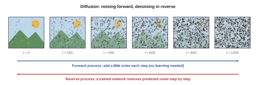
A diffusion model learns to reverse a gradual noising process. In the forward process, which needs no learning, a training image is corrupted step by step with small amounts of Gaussian noise until, after many steps, nothing but noise remains. At step \( t \) the noisy image can be written directly as:
Here \( x_0 \) is the clean image and \( \bar\alpha_t \) falls from nearly 1 to nearly 0 according to a noise schedule. A neural network, typically a U-Net or, in newer models, a transformer, is trained to predict the noise \( \varepsilon \) that was added, given \( x_t \) and \( t \). Once trained, generation runs backward: start from pure random noise and repeatedly use the network to remove a little predicted noise, step by step, until a clean image emerges. Jonathan Ho and colleagues' 2020 paper on denoising diffusion probabilistic models (DDPM) made the approach practical; later work cut the number of steps from about 1,000 to between roughly 4 and 50 using better samplers and distillation.
There is a satisfying link to the rest of this course: a diffusion model is, at heart, a very powerful learned denoiser applied repeatedly. Early steps decide the overall composition and colours, because at high noise only coarse structure can be inferred; late steps add fine detail and texture. This is why changing the random seed changes the whole composition, while some editing techniques, such as image-to-image generation, start partway through the process from a noised version of an existing photo to keep its composition.
import numpy as np
rng = np.random.default_rng(420)
modes = np.array([-2.0, 2.0]); s = 0.3; weights = np.array([0.7, 0.3])  # the "training data": two clusters
def score(x, sigma):
    var = s ** 2 + sigma ** 2
    logp = -((x[:, None] - modes) ** 2) / (2 * var) + np.log(weights)
    r = np.exp(logp - logp.max(axis=1, keepdims=True)); r /= r.sum(axis=1, keepdims=True)
    return (r * (modes - x[:, None])).sum(axis=1) / var
sigmas = np.geomspace(10, 0.01, 60)                 # noise levels from high to low
x = rng.normal(0, sigmas[0], 5000)                  # start from pure noise
for sig in sigmas:
    step = 0.1 * sig ** 2
    for _ in range(5):                              # a few Langevin steps per noise level
        x = x + step * score(x, sig) + np.sqrt(2 * step) * rng.normal(size=x.size)
near_left = np.mean(np.abs(x + 2) < 1); near_right = np.mean(np.abs(x - 2) < 1)
print(f"start: spread {sigmas[0]:.0f}; end: {near_left * 100:.1f} % near -2, {near_right * 100:.1f} % near +2")
print(f"spread within the left cluster: {x[np.abs(x + 2) < 1].std():.2f} (data {s})")start: spread 10; end: 66.6 % near -2, 32.7 % near +2 spread within the left cluster: 0.33 (data 0.3)
Starting from noise spread over a wide range, repeated small denoising steps guided by the score (the direction toward higher probability at each noise level) end with samples that reproduce the locations and spread of the two clusters and, approximately, their 70:30 balance (about 67:33 in this run). A real image model does the same in hundreds of thousands of dimensions, with a neural network estimating the score instead of an exact formula.
Steering with text: conditioning and guidance
Text-to-image models condition the denoising network on a representation of the prompt. Early systems used text encoders trained to match images and captions, such as OpenAI's CLIP (2021), which learned from about 400 million image-caption pairs to place matching images and texts near each other in a shared embedding space. Newer systems use large language model encoders, which understand longer and more precise prompts. The network sees the text embedding at every step through attention layers, so words influence which features appear where.
Classifier-free guidance strengthens the effect of the prompt. At each step the network makes two predictions, one with the prompt and one without, and the sampler extrapolates away from the unconditional prediction:
The guidance scale \( w \) trades fidelity to the prompt against variety and naturalness. Values around 5 to 8 were common for Stable Diffusion-style models; very high values give saturated, over-contrasted images. Negative prompts replace the unconditional prediction with one conditioned on unwanted features, steering away from them. Many current commercial systems hide these controls and tune them internally.
Worked problem
Applying classifier-free guidance
At one step and one pixel, the unconditional noise prediction is 0.20 and the conditional prediction is 0.30. Compute the guided prediction for \( w = 1 \), 4 and 8.
Show solution
- Difference: \( 0.30 - 0.20 = 0.10 \).
- \( w = 1 \): \( 0.20 + 0.10 = 0.30 \), the plain conditional prediction.
- \( w = 4 \): \( 0.20 + 0.40 = 0.60 \); \( w = 8 \): \( 0.20 + 0.80 = 1.00 \).
Answer: 0.30, 0.60 and 1.00; larger \( w \) pushes the prediction further in the direction the prompt suggests, which can exaggerate features.
| Setting | What it controls | Too low | Too high |
|---|---|---|---|
| Steps | Number of denoising iterations | Unfinished, noisy or smeared | Slower with little gain |
| Guidance scale | Strength of prompt adherence | Ignores the prompt | Oversaturated, harsh, repetitive |
| Seed | Starting noise | Not applicable | Not applicable; changes composition |
| Image-to-image strength | How far to noise the input | Little change | Input composition lost |
| Resolution | Output pixel dimensions | Low detail | Duplicated subjects if beyond training size |
Transformers, flow matching and autoregressive models
Image generation changes quickly. Since about 2023, many leading models replaced the U-Net with diffusion transformers (DiT), which scale better with compute, and adopted flow matching or rectified flow, related training methods that learn straighter paths from noise to image and need fewer steps. Some systems generate images autoregressively, predicting image tokens one after another like a language model, often within multimodal models that can both understand and edit images in conversation. From the photographer's point of view, the practical results are better prompt understanding, legible text in images, more consistent characters across images, and editing by instruction ("make it golden hour", "remove the people") rather than by masks and sliders. Model names and capabilities change monthly; the principles above change slowly.
Inpainting, outpainting and generative fill
Inpainting regenerates a masked region of an existing image so that it blends with its surroundings. The model sees the unmasked pixels and the mask and generates only the masked area, consistent with the context and an optional prompt. Outpainting, or generative expand, extends an image beyond its borders. Adobe's Generative Fill in Photoshop (2023), built on Adobe's Firefly models, made these techniques mainstream for photographers, and similar features exist in many editors and phones: removing distractions, replacing skies, changing clothing, extending backgrounds for different aspect ratios. Traditional content-aware fill, available since 2010, copied patches from elsewhere in the same image; generative fill invents new content from training, which handles complex areas far better and also makes it possible to add things that were never there.
Other control techniques give photographers more precision. Image-to-image generation starts from a noised version of an input photo, preserving its composition at low strength. ControlNet-style conditioning (2023) guides generation with edge maps, depth maps or human poses extracted from a reference. Low-rank adaptation (LoRA) fine-tunes a model on a small set of images, perhaps 10 to 50, to learn a specific product, person or style, which is powerful for product photography and also raises consent and likeness issues covered in lessons 10 and 11.
Training data and its consequences
Generative models learn from enormous datasets. LAION-5B, released in 2022, contained about 5.85 billion image-text pairs scraped from the web and was used to train several open models; it was later found to contain links to illegal and private material and was temporarily withdrawn and cleaned in 2024. Other developers trained on licensed or owned collections: Adobe states that Firefly was trained on Adobe Stock and other licensed or public-domain content, and Getty Images and Shutterstock launched generators trained on their libraries with contributor compensation schemes (company statements; terms change). Training data shapes everything a model produces: its aesthetic defaults, its biases in depicting people and places, the styles it can imitate and the legal questions it raises. Whether training on copyrighted photographs without permission is lawful is being litigated in several countries; lesson 11 summarizes the position at the time of writing.
steps = 30
seconds_per_step = 0.05          # on a server GPU at 1,024 px (assumed)
gpu_watts = 700                  # assumed board power
images = 1000
t_per_image = steps * seconds_per_step
kwh = t_per_image * images * gpu_watts / 3.6e6
print(f"{t_per_image:.1f} s per image, {t_per_image * images / 60:.0f} GPU-minutes for {images} images")
print(f"about {kwh:.2f} kWh of GPU energy (excluding cooling, idle time and training)")
for s in (4, 8, 50):
print(f"{s:2d} steps: {s * seconds_per_step:.2f} s per image")1.5 s per image, 25 GPU-minutes for 1000 images about 0.29 kWh of GPU energy (excluding cooling, idle time and training) 4 steps: 0.20 s per image 8 steps: 0.40 s per image 50 steps: 2.50 s per image
Inference costs for a single image are modest under these assumptions, but they scale with billions of images generated daily, and training a large model consumes far more. Distilled models that generate in a few steps cut inference costs sharply. Environmental impact is part of the ethical picture discussed in lesson 10.
What generative models still get wrong
Generative models have improved rapidly, but characteristic weaknesses persist to varying degrees: physically inconsistent lighting and shadows, reflections that do not match, perspective errors in architecture, garbled small text and logos in some models, anatomical errors in hands and teeth (much reduced in recent models), repeated textures and an overly polished "AI look" with idealized faces. These flaws are not reliable detection signals, because each model generation fixes some of them, but they matter for quality control in professional work. Lesson 11 explains why visual inspection and automated detectors are weak tools for proving whether an image is generated, and why provenance records are a stronger approach.
Common mistakes
MistakeThinking a generative model retrieves or collages training images
InsteadUnderstand that it samples new images from a learned distribution, though it can sometimes reproduce memorized training images.
MistakeAssuming more guidance always means better prompt following
InsteadUse moderate guidance; high values cause oversaturation and artefacts.
MistakeTreating generative fill as the same as content-aware fill
InsteadRemember generative fill invents content from training, while content-aware fill copies from the same image.
MistakeFine-tuning on a person's likeness without consent
InsteadObtain consent and releases before training or generating identifiable people.
MistakeRelying on visual flaws to spot AI images
InsteadExpect flaws to disappear with new models and use provenance instead.
Summary and key terms
- Generative models learn the distribution of images and sample new ones, unlike restorative models anchored to an input.
- Latent spaces compress images so that generation is cheaper; decoders restore pixels.
- GANs pit a generator against a discriminator; diffusion models learn to reverse gradual noising.
- Diffusion is a powerful learned denoiser applied repeatedly from pure noise, coarse structure first and detail last.
- Text conditioning and classifier-free guidance steer generation; guidance trades adherence for naturalness.
- Inpainting, outpainting, image-to-image, ControlNet and LoRA give fine control over edits and subjects.
- Training data shapes style, bias and legal risk, and compute has environmental costs.
- Generative model
- A model that learns a data distribution and samples new examples from it.
- Latent space
- A compressed representation in which images are encoded for efficient generation.
- Generative adversarial network (GAN)
- A generator and discriminator trained in competition to produce realistic images.
- Diffusion model
- A model that generates by reversing a gradual noising process with a learned denoiser.
- Noise schedule
- The plan for how much noise is present at each diffusion step.
- Classifier-free guidance
- Extrapolating from unconditional toward conditional predictions to strengthen prompt adherence.
- CLIP
- A model that embeds images and text in a shared space, used to condition early text-to-image systems.
- Inpainting
- Regenerating a masked region to blend with the rest of an image.
- LoRA
- Low-rank adaptation, an efficient way to fine-tune a model on a small set of images.
- ControlNet
- A method for conditioning generation on structural guides such as edges, depth or poses.
Practice problems
Work each problem on paper first, then reveal the answer to check.
What is the key difference between a restorative and a generative model?
Show answer
A restorative model is anchored to an input photo; a generative model samples new images from its learned distribution.
A 512 by 512 RGB image is encoded as 64 by 64 by 4. What is the reduction factor?
Show answer
\( 786\,432 / 16\,384 = 48 \).
What do the two networks in a GAN do?
Show answer
The generator creates images; the discriminator tries to tell them from real ones.
In diffusion, what does the network learn to predict?
Show answer
The noise added to an image at a given step.
Why does changing the seed change the whole composition?
Show answer
The starting noise determines coarse structure, which is decided in early steps.
Unconditional 0.1, conditional 0.25, guidance 6. Guided value?
Show answer
\( 0.1 + 6 \times 0.15 = 1.0 \).
How does generative fill differ from content-aware fill?
Show answer
It generates new content from a trained model rather than copying patches from the same image.
What does image-to-image strength control?
Show answer
How much noise is added to the input before denoising, and so how much the composition changes.
What is LoRA used for in photography workflows?
Show answer
Fine-tuning a model on a small set of images of a product, person or style.
Why are visual flaws unreliable for detecting AI images?
Show answer
New models fix them, and real photos can show similar artefacts.
Lesson quiz · 5 questions
Score 60% or more to complete this lesson.
Create a free account to save your progress, take quizzes and earn a certificate.