
ROB-210 · Lesson 10 of 12 · 32 min
Velocity kinematics and the Jacobian
Robots move, so knowing where the tool is matters less than knowing how fast it is going and how to make it go where we want at a controlled speed. Velocity kinematics relates joint velocities to the tool's linear and angular velocity through the Jacobian matrix. The Jacobian is arguably the most important object in robot kinematics: it drives Cartesian motion control, numerical inverse kinematics, force control and collision avoidance; it reveals singularities; and its transpose maps forces at the tool to torques at the joints. This lesson defines the Jacobian carefully, shows how to compute it for any serial arm, and connects velocity to static force.
From positions to velocities
Forward kinematics gives the tool pose as a function of the joints, \( \mathbf{x} = f(\mathbf{q}) \). Differentiating with respect to time using the chain rule gives the relationship between velocities:
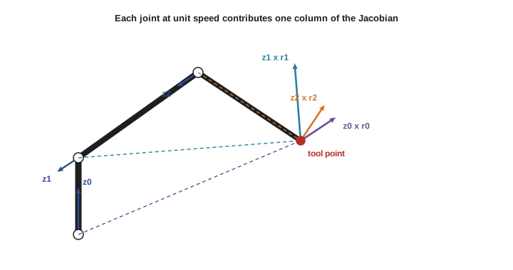
The relationship is linear in the joint velocities, which is what makes the Jacobian so useful, but the matrix itself depends on the configuration. Column i of J is the tool velocity produced when joint i moves at unit speed and all others are still. For a planar 2R arm with link lengths \( L_1 \) and \( L_2 \), differentiating \( x = L_1c_1 + L_2c_{12} \) and \( y = L_1s_1 + L_2s_{12} \) gives:
Worked problem
Tool velocity of a 2R arm
A 2R arm with \( L_1 = 0.4 \) and \( L_2 = 0.3 \) m is at \( \boldsymbol{\theta} = (30^\circ, 60^\circ) \). The shoulder turns at 0.5 rad/s and the elbow at −0.2 rad/s. Find the tool velocity.
Show solution
- \( s_1 = 0.5 \), \( c_1 = 0.866 \), \( s_{12} = \sin 90^\circ = 1 \), \( c_{12} = 0 \).
- \( J = \begin{bmatrix} -0.2 - 0.3 & -0.3 \\ 0.346 + 0 & 0 \end{bmatrix} = \begin{bmatrix} -0.5 & -0.3 \\ 0.346 & 0 \end{bmatrix} \).
- \( \dot{x} = -0.5(0.5) - 0.3(-0.2) = -0.25 + 0.06 = -0.19 \) m/s; \( \dot{y} = 0.346(0.5) = 0.173 \) m/s.
Answer: The tool moves at (−0.19, 0.173) m/s, a speed of about 0.26 m/s. Because the forearm points straight up here, the elbow joint can move the tool only sideways, which shows in the zero in the second column.
Twists: linear and angular velocity together
In three dimensions, the tool's motion has a linear part, the velocity \( \mathbf{v} \) of the tool point, and an angular part, the angular velocity \( \boldsymbol{\omega} \) of the tool frame. Together they form a six-dimensional twist. The geometric Jacobian is the 6 × n matrix that maps joint velocities to this twist:
Different books stack the parts in different orders: Siciliano and Spong put linear velocity first, as here, while Lynch and Park put angular velocity first, matching their (ω, v) screw axes. Neither is wrong, but mixing conventions between a textbook formula and a library produces rows in the wrong place, so check before combining. Angular velocity has a subtlety: it is not the time derivative of any set of three angles. It is a vector describing the instantaneous axis and rate of rotation, related to the derivative of the rotation matrix by \( \dot{R} = [\boldsymbol{\omega}]R \).
Computing the geometric Jacobian column by column
There is a simple geometric construction for each column. Let \( \hat{\mathbf{z}}_{i-1} \) be the axis of joint i and \( \mathbf{p}_{i-1} \) a point on it, both in the base frame at the current configuration, and let \( \mathbf{p}_e \) be the tool point. Then:
The revolute formula is the velocity of a point on a rotating body from lesson 1, \( \boldsymbol{\omega} \times \mathbf{r} \), with unit rotation speed; a revolute joint also contributes angular velocity along its axis. A prismatic joint moves the tool along its axis without rotating it. With DH frames, \( \hat{\mathbf{z}}_{i-1} \) and \( \mathbf{p}_{i-1} \) are simply the third and fourth columns of \( {}^{0}T_{i-1} \), which the forward kinematics computes anyway, so building the Jacobian adds very little cost.
In the product of exponentials framework, the space Jacobian has an even neater form: its first column is the screw axis \( \mathcal{S}_1 \), and column i is \( \mathcal{S}_i \) transformed by the motion of the joints before it, \( [\mathrm{Ad}_{e^{[\mathcal{S}_1]\theta_1} \cdots e^{[\mathcal{S}_{i-1}]\theta_{i-1}}}]\,\mathcal{S}_i \). In words, each column is the current screw axis of that joint. The space Jacobian gives the twist expressed in the base frame and referred to the base origin, which differs from the geometric Jacobian's tool-point velocity by a simple change of reference point.
Worked problem
A column of the geometric Jacobian
At some configuration, joint 2 of an arm has axis \( \hat{\mathbf{z}}_1 = (0, -1, 0) \) through \( \mathbf{p}_1 = (0, 0, 0.3) \), and the tool is at \( \mathbf{p}_e = (0.5, 0, 0.6) \) m. Find the Jacobian column for joint 2.
Show solution
- \( \mathbf{r} = \mathbf{p}_e - \mathbf{p}_1 = (0.5, 0, 0.3) \).
- \( \hat{\mathbf{z}}_1 \times \mathbf{r} = ((-1)(0.3) - 0 \cdot 0,\; 0 \cdot 0.5 - 0 \cdot 0.3,\; 0 \cdot 0 - (-1)(0.5)) = (-0.3, 0, 0.5) \).
- Column: \( J_2 = (-0.3, 0, 0.5,\; 0, -1, 0) \).
Answer: Turning joint 2 at 1 rad/s moves the tool at (−0.3, 0, 0.5) m/s, back and up, and rotates it at 1 rad/s about −y. Its length, 0.58 m/s, equals the distance from the axis to the tool.
Geometric versus analytic Jacobian
If the orientation part of the task is described by three angles \( \boldsymbol{\phi} \), such as roll-pitch-yaw, we can differentiate the forward kinematics with respect to those angles directly. That gives the analytic Jacobian \( J_a \), relating \( \dot{\mathbf{q}} \) to \( (\dot{\mathbf{p}}, \dot{\boldsymbol{\phi}}) \). It differs from the geometric Jacobian because angle rates are not angular velocity. The two are linked by a matrix that depends on the angles:
For roll-pitch-yaw, \( B \) becomes singular at pitch ±90°, the gimbal lock of lesson 3. These representation singularities are artefacts of the chosen angles, not physical limitations of the robot, and they are one reason most controllers work with the geometric Jacobian and rotation-vector errors rather than angle rates. The analytic Jacobian is still useful when a task is naturally specified in angles, for example keeping a camera's roll at zero while it pans and tilts.
| Jacobian | Maps \( \dot{\mathbf{q}} \) to | Typical use | Watch for |
|---|---|---|---|
| Geometric | Tool-point velocity and angular velocity, base frame | Cartesian control, IK, statics | Ordering of linear and angular rows |
| Space (PoE) | Twist in base frame, referred to the base origin | Screw-theory analysis | Reference point differs from the tool point |
| Body (PoE) | Twist in the tool frame | Tool-centred tasks, force control at the tool | Frame of expression |
| Analytic | Position rates and orientation angle rates | Tasks specified in angles | Representation singularities |
Using the Jacobian for motion control
Inverting the velocity relationship gives the joint velocities needed for a desired tool velocity:
This is resolved-rate motion control, proposed by Whitney in 1969. At each control cycle, perhaps every 2 ms, the controller computes the Jacobian at the current configuration, solves for the joint velocities that produce the desired tool velocity, and commands them. Adding a correction proportional to the pose error, \( \dot{\mathbf{x}} = \dot{\mathbf{x}}_d + K(\mathbf{x}_d - \mathbf{x}) \), keeps the tool on its path despite numerical drift, and the numerical IK of lesson 9 is essentially this loop run to convergence without real time passing. It is how a robot moves its tool in a straight line, how a teleoperated arm follows a hand controller, and how ROS 2's MoveIt Servo jogs an arm in Cartesian space.
Worked problem
Joint speeds for a straight-line motion
The 2R arm of the first example, at \( (30^\circ, 60^\circ) \), must move its tool straight up at 0.1 m/s. Find the joint velocities.
Show solution
- Solve \( \begin{bmatrix} -0.5 & -0.3 \\ 0.346 & 0 \end{bmatrix} \begin{bmatrix} \dot{\theta}_1 \\ \dot{\theta}_2 \end{bmatrix} = \begin{bmatrix} 0 \\ 0.1 \end{bmatrix} \).
- Second row: \( \dot{\theta}_1 = 0.1/0.346 = 0.289 \) rad/s.
- First row: \( -0.5(0.289) - 0.3\dot{\theta}_2 = 0 \), so \( \dot{\theta}_2 = -0.481 \) rad/s.
Answer: About 0.29 rad/s at the shoulder and −0.48 rad/s at the elbow. These speeds change continuously as the arm moves, so the controller recomputes them every cycle.
Statics: the Jacobian transpose
The Jacobian also governs forces. If the tool pushes on its environment with a force \( \mathbf{f} \) and a moment \( \mathbf{m} \), together called a wrench \( \mathcal{F} \), the joint torques needed to hold it in static equilibrium are:
This follows from the principle of virtual work: the power delivered at the joints, \( \boldsymbol{\tau}^\mathsf{T}\dot{\mathbf{q}} \), must equal the power delivered at the tool, \( \mathcal{F}^\mathsf{T}\dot{\mathbf{x}} = \mathcal{F}^\mathsf{T}J\dot{\mathbf{q}} \), for every joint velocity. The relation is used to size motors for a required payload or push force, to estimate contact forces from measured joint torques in collaborative robots, and in impedance and force control, covered in ROB-300. It also explains a familiar experience: when your arm is nearly straight you can support a large load along the arm with little effort, because the Jacobian makes that direction cheap in torque, while pushing sideways is hard.
Worked problem
Joint torques to hold a payload
The 2R arm at \( (30^\circ, 60^\circ) \) holds a 2 kg mass at its tool, so the tool must apply an upward force of \( 2 \times 9.81 = 19.6 \) N. Ignoring link weights, what torques do the joints need?
Show solution
- Wrench (planar force only): \( \mathbf{f} = (0, 19.6) \) N.
- \( J^\mathsf{T} = \begin{bmatrix} -0.5 & 0.346 \\ -0.3 & 0 \end{bmatrix} \).
- \( \boldsymbol{\tau} = J^\mathsf{T}\mathbf{f} = (0.346 \times 19.6,\; 0) = (6.8, 0) \) N·m.
Answer: The shoulder needs 6.8 N·m and the elbow none, because the forearm points straight up and the load acts along it. This is the same column structure that made the elbow unable to move the tool vertically in the first example: directions of zero motion are directions of free support.
Computing and checking Jacobians in code
A numerical Jacobian, obtained by perturbing each joint slightly and differencing the forward kinematics, is a valuable test of an analytic one. The listing builds the geometric Jacobian of an elbow arm from its DH frames, using the column formula above, and compares its position rows with central differences.
import numpy as np
np.set_printoptions(precision=4, suppress=True)
def dh(t, d, a, al):
    ct, st, ca, sa = np.cos(t), np.sin(t), np.cos(al), np.sin(al)
    return np.array([[ct,-st*ca,st*sa,a*ct],[st,ct*ca,-ct*sa,a*st],[0,sa,ca,d],[0,0,0,1]])
TABLE = [(0.30, 0.0, np.pi/2), (0.0, 0.40, 0.0), (0.0, 0.35, 0.0)]   # (d, a, alpha) of an elbow arm
def frames(q):
    Ts, T = [np.eye(4)], np.eye(4)
    for qi, (d, a, al) in zip(q, TABLE):
        T = T @ dh(qi, d, a, al); Ts.append(T)
    return Ts
def jacobian(q):
    Ts = frames(q); pe = Ts[-1][:3, 3]
    cols = [np.hstack([np.cross(T[:3,2], pe - T[:3,3]), T[:3,2]]) for T in Ts[:-1]]
    return np.array(cols).T
q = np.radians([45, 30, -60])
J = jacobian(q)
print("geometric Jacobian (v rows then w rows):\n", J)
h = 1e-6
Jnum = np.array([(frames(q + h*e)[-1][:3,3] - frames(q - h*e)[-1][:3,3]) / (2*h) for e in np.eye(3)]).T
print("max difference from finite differences:", f"{np.abs(J[:3] - Jnum).max():.1e}")geometric Jacobian (v rows then w rows): [[-0.4593 -0.0177 0.1237] [ 0.4593 -0.0177 0.1237] [ 0. 0.6495 0.3031] [ 0. 0.7071 0.7071] [ 0. -0.7071 -0.7071] [ 1. 0. 0. ]] max difference from finite differences: 7.6e-11
Common mistakes
MistakeTreating angular velocity as the derivative of Euler angles.
InsteadAngular velocity is a vector; relate it to angle rates with \( \boldsymbol{\omega} = B(\boldsymbol{\phi})\dot{\boldsymbol{\phi}} \).
MistakeMixing (v, ω) and (ω, v) row orderings.
InsteadCheck the convention of each formula and library before combining them.
MistakeUsing a Jacobian computed at an old configuration.
InsteadRecompute J every control cycle; it changes as the robot moves.
MistakeForgetting the reference point of a twist.
InsteadThe geometric Jacobian gives the tool-point velocity; the space Jacobian refers to the base origin.
MistakeUsing J instead of its transpose for statics.
InsteadJoint torques are \( \boldsymbol{\tau} = J^\mathsf{T}\mathcal{F} \).
Summary and key terms
- The Jacobian maps joint velocities linearly to tool velocities: \( \dot{\mathbf{x}} = J(\mathbf{q})\dot{\mathbf{q}} \).
- Each column is the tool velocity from one joint at unit speed.
- Geometric Jacobian columns are \( (\hat{\mathbf{z}} \times \mathbf{r}, \hat{\mathbf{z}}) \) for revolute joints and \( (\hat{\mathbf{z}}, \mathbf{0}) \) for prismatic ones.
- In PoE, space Jacobian columns are the current screw axes of the joints.
- The analytic Jacobian uses angle rates and inherits representation singularities.
- Resolved-rate control computes \( \dot{\mathbf{q}} = J^{-1}\dot{\mathbf{x}}_d \) (or \( J^{+} \)) every cycle.
- Statics: joint torques balancing a tool wrench are \( \boldsymbol{\tau} = J^\mathsf{T}\mathcal{F} \).
- Velocity kinematics
- The relationship between joint velocities and tool velocities.
- Geometric Jacobian
- The matrix mapping joint velocities to tool linear and angular velocity.
- Angular velocity
- A vector giving the instantaneous axis and rate of rotation of a body.
- Space Jacobian
- The PoE Jacobian giving the twist in the base frame.
- Body Jacobian
- The PoE Jacobian giving the twist in the tool frame.
- Analytic Jacobian
- The derivative of a pose described by position and three angles.
- Resolved-rate control
- Commanding joint velocities from desired tool velocities through the inverse Jacobian.
- Wrench
- A combined force and moment acting on a body.
- Virtual work
- The principle that equates joint power and tool power, giving \( \boldsymbol{\tau} = J^\mathsf{T}\mathcal{F} \).
- Finite differences
- Approximating derivatives by evaluating a function at slightly perturbed inputs.
Practice problems
Work each problem on paper first, then reveal the answer to check.
What shape is the geometric Jacobian of a 6-joint arm?
Show answer
6 × 6.
A 2R arm with \( L_1 = L_2 = 1 \) m is at (0°, 0°). Write J.
Show answer
\( \begin{bmatrix} 0 & 0 \\ 2 & 1 \end{bmatrix} \).
In that pose, can the tool move along x?
Show answer
No; the first row is zero, so the arm is at a singularity for x motion.
A revolute axis is z = (0, 0, 1) through the origin; the tool is at (1, 0, 0). Find the linear part of its column.
Show answer
\( (0,0,1) \times (1,0,0) = (0, 1, 0) \).
What is the angular part of a prismatic joint's column?
Show answer
Zero.
A tool must move at (0, 0.1) m/s and \( J = \begin{bmatrix} -0.5 & -0.3 \\ 0.346 & 0 \end{bmatrix} \). What is \( \dot{\theta}_1 \)?
Show answer
0.289 rad/s.
Write the static torque relation.
Show answer
\( \boldsymbol{\tau} = J^\mathsf{T}\mathcal{F} \).
A 2R arm's \( J^\mathsf{T} \) row for the elbow is (−0.3, 0). What elbow torque holds a 10 N force along x?
Show answer
−3 N·m.
Why might a controller avoid the analytic Jacobian?
Show answer
Angle rates have representation singularities, such as gimbal lock.
How can you test an analytic Jacobian?
Show answer
Compare it with finite differences of the forward kinematics.
Lesson quiz · 5 questions
Score 60% or more to complete this lesson.
Create a free account to save your progress, take quizzes and earn a certificate.