
ROB-210 · Lesson 8 of 12 · 29 min
Inverse kinematics: analytical methods
Robots are usually told what to do in terms of the tool: pick the part at this position, hold the camera at that orientation, follow this weld seam. The controller, however, can only command joints. Inverse kinematics (IK) bridges the gap by finding joint values that put the tool at a desired pose. Unlike forward kinematics, IK can have no solution (the target is out of reach), several solutions (the arm can reach the same pose with the elbow up or down), or infinitely many (a redundant arm). For many arm designs, IK can be solved exactly with geometry and trigonometry, giving all solutions in microseconds with no iteration. This lesson develops those analytical, or closed-form, methods.
Why analytical solutions are valuable
An analytical IK solution is a set of formulas that compute the joint angles directly. Compared with the numerical methods of lesson 9, closed-form solutions are faster and more predictable: they take a fixed, small amount of time, they never fail to converge, and they return every solution, so the controller can choose the most suitable one. This matters for real-time control, for planning, which may call IK millions of times, and for safety, because the robot can avoid unexpected jumps between solution branches. The price is that closed-form solutions exist only for certain geometries and must be derived for each robot design. Pieper showed in 1968 that a six-joint arm has a closed-form solution if three consecutive joint axes intersect at a point, as in a spherical wrist, or are parallel. Most industrial arms are designed to satisfy this condition precisely so that their IK can be solved analytically.
The planar 2R arm
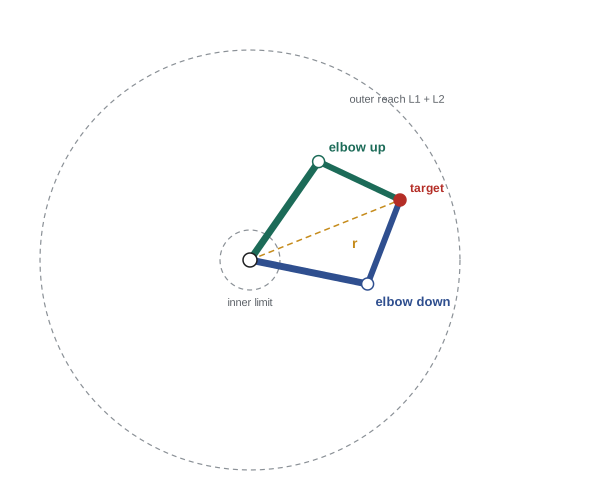
The planar two-link arm is the foundation for almost every analytical solution. Given a target \( (x, y) \) and link lengths \( L_1 \) and \( L_2 \), we want \( \theta_1 \) and \( \theta_2 \). The distance from the shoulder to the target, \( r = \sqrt{x^2 + y^2} \), and the two links form a triangle. The law of cosines gives the elbow angle:
If \( |D| > 1 \), no triangle exists and the target is unreachable: either too far, beyond \( L_1 + L_2 \), or too close, inside \( |L_1 - L_2| \). Otherwise the two signs of the square root give the two solutions, elbow down and elbow up, which are mirror images about the line from shoulder to target. With \( \theta_2 \) known, the shoulder angle is the direction to the target minus the angle the forearm adds:
Using atan2 rather than arccos or arctan handles all quadrants correctly and avoids the precision loss of arccos near 0° and 180°. When \( D = \pm 1 \), the two solutions merge: the arm is fully stretched or fully folded, a boundary singularity examined in lesson 11.
Worked problem
Solving a 2R arm
A planar arm has \( L_1 = 0.4 \) m and \( L_2 = 0.3 \) m. Find both solutions that reach \( (0.5, 0.2) \) m.
Show solution
- \( x^2 + y^2 = 0.25 + 0.04 = 0.29 \). \( D = (0.29 - 0.16 - 0.09)/(2 \times 0.4 \times 0.3) = 0.04/0.24 = 0.1667 \).
- \( \sqrt{1 - D^2} = 0.986 \), so \( \theta_2 = \pm 80.4^\circ \).
- Direction to target: \( \operatorname{atan2}(0.2, 0.5) = 21.8^\circ \).
- For \( \theta_2 = +80.4^\circ \): \( \operatorname{atan2}(0.3 \times 0.986,\; 0.4 + 0.3 \times 0.1667) = \operatorname{atan2}(0.296, 0.450) = 33.3^\circ \), so \( \theta_1 = -11.5^\circ \).
- For \( \theta_2 = -80.4^\circ \): \( \theta_1 = 21.8^\circ + 33.3^\circ = 55.1^\circ \).
Answer: Elbow down: (−11.5°, 80.4°); elbow up: (55.1°, −80.4°). Substituting either pair into the forward kinematics returns (0.5, 0.2), which is always the final check.
Adding orientation: the planar 3R arm
A planar 3R arm can also control the tool's heading \( \phi \). The trick is to work backwards from the tool to the wrist, the end of link 2, which must lie a distance \( L_3 \) behind the tool along its heading:
Solving the 2R problem for the wrist gives \( \theta_1 \) and \( \theta_2 \), and the last joint supplies whatever rotation remains: \( \theta_3 = \phi - \theta_1 - \theta_2 \). This 'subtract the last link, solve the rest' idea is a miniature version of the wrist decoupling used for six-axis arms.
Worked problem
Planar 3R with heading
The arm of lesson 5 (\( L_1 = 0.4 \), \( L_2 = 0.3 \), \( L_3 = 0.1 \) m) must place its tool at \( (0.521, 0.516) \) m with heading 15°. Find the elbow-down solution.
Show solution
- Wrist: \( x_w = 0.521 - 0.1\cos 15^\circ = 0.424 \), \( y_w = 0.516 - 0.1\sin 15^\circ = 0.490 \).
- 2R: \( D = (0.424^2 + 0.490^2 - 0.25)/0.24 = (0.180 + 0.240 - 0.25)/0.24 \approx 0.709 \), so \( \theta_2 \approx 44.8^\circ \).
- \( \theta_1 = \operatorname{atan2}(0.490, 0.424) - \operatorname{atan2}(0.211, 0.613) \approx 49.1^\circ - 19.0^\circ = 30.1^\circ \).
- \( \theta_3 = 15^\circ - 30.1^\circ - 44.8^\circ = -59.9^\circ \).
Answer: About (30°, 45°, −60°), the angles used in the forward kinematics example of lesson 5; the small differences come from rounding the tool position to three decimals. Inverse kinematics followed by forward kinematics returns the original pose.
The elbow arm in three dimensions
For the elbow arm of lesson 6, the wrist centre \( (x, y, z) \) is reached by the first three joints. The waist angle points the arm's vertical plane at the target, and then the shoulder and elbow solve a planar 2R problem in that plane:
The planar problem has target \( (r, s) \) with link lengths \( a_2 \) and \( a_3 \), giving two elbow solutions. There is a second waist solution too: the arm can turn to face away from the target, \( \theta_1 + 180^\circ \), and reach back over its own shoulder with \( r \) replaced by \( -r \). This 'shoulder left' versus 'shoulder right' choice, combined with elbow up or down, gives four solutions for the position of the wrist. If the wrist centre lies on the waist axis, where \( x = y = 0 \), \( \theta_1 \) is undefined: any waist angle works. This shoulder singularity needs special handling in software.
Worked problem
Solving an elbow arm for the wrist centre
With \( d_1 = 0.30 \), \( a_2 = 0.40 \) and \( a_3 = 0.35 \) m, find the solutions facing the target that put the wrist at \( (0.460, 0.460, 0.325) \) m, the point from lesson 6.
Show solution
- \( \theta_1 = \operatorname{atan2}(0.460, 0.460) = 45^\circ \); \( r = 0.650 \), \( s = 0.025 \).
- \( D = (0.650^2 + 0.025^2 - 0.16 - 0.1225)/(2 \times 0.4 \times 0.35) = (0.4238 - 0.2825)/0.28 \approx 0.505 \), so \( \theta_3 \approx \pm 59.7^\circ \).
- For \( \theta_3 = -59.7^\circ \): \( \theta_2 = \operatorname{atan2}(0.025, 0.650) + \operatorname{atan2}(0.302, 0.577) \approx 2.2^\circ + 27.7^\circ = 29.9^\circ \).
- For \( \theta_3 = +59.7^\circ \): \( \theta_2 \approx 2.2^\circ - 27.7^\circ = -25.5^\circ \).
Answer: Elbow up: about (45°, 30°, −60°), recovering lesson 6's pose to within the rounding of the wrist position; elbow down: about (45°, −25.5°, 60°). Two more solutions use \( \theta_1 = -135^\circ \) and reach backwards, if the joint limits allow.
Wrist decoupling for six-axis arms
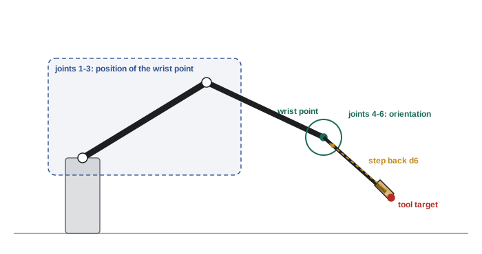
For a six-axis arm with a spherical wrist, Pieper's condition lets us split the problem in two. Given the desired tool pose, with orientation R and position p, and a tool length \( d_6 \) along the approach axis:
- Find the wrist centre by stepping back from the tool along its approach direction: \( \mathbf{p}_w = \mathbf{p} - d_6 R\,\hat{\mathbf{z}} \).
- Solve the first three joints for the wrist centre, as above, giving up to four solutions.
- For each, compute the orientation the wrist must supply: \( {}^{3}R_{6} = ({}^{0}R_{3})^\mathsf{T} R \), using the forward kinematics of the first three joints.
- Extract the three wrist angles from \( {}^{3}R_{6} \) as Euler angles, typically Z-Y-Z, giving two solutions each (wrist flipped or not).
Together this yields up to eight solutions for a classic six-axis arm such as the PUMA 560 design: shoulder left or right, elbow up or down, wrist flipped or not flipped. Industrial controllers expose this choice as a configuration flag stored with each taught point, so that a program always reaches a point in the same arrangement. Moving between configurations requires passing through a singularity, so the planner must handle such transitions deliberately.
| Arm type | Typical number of IK solutions | Notes |
|---|---|---|
| Planar 2R | 2 (elbow up, elbow down) | Merge at full stretch or fold |
| Planar 3R with heading | 2 | Wrist point found first |
| SCARA | 2 | Vertical axis and tool roll decoupled |
| Elbow arm (position only) | 4 | Shoulder left/right times elbow up/down |
| Six-axis, spherical wrist | Up to 8 | Plus wrist flip; extra multiples of 360° if joints exceed ±180° |
| General six-axis (no special geometry) | Up to 16 | Needs polynomial or numerical methods |
| Seven-axis redundant | Infinitely many | A one-parameter family; choose with an extra criterion |
Arms without a spherical wrist
Collaborative arms like the UR series use offset wrists, so the wrist centre is not a single point. They nonetheless satisfy Pieper's condition in a different way: joints 2, 3 and 4 are parallel. Published analytical solutions exist for this family and also give up to eight solutions. A general six-axis arm with no special geometry can have up to sixteen solutions, found by reducing the equations to a single polynomial of degree sixteen; this was a celebrated result of kinematics research around 1990, but in practice such arms are rare precisely because their IK is awkward.
Deriving closed forms by hand is error-prone, so tools exist to automate it. IKFast, part of the OpenRAVE project, generates C++ solver code from a robot description, and MoveIt can use the generated plugins; other tools such as IKFlow, TRAC-IK and the analytic solvers supplied by manufacturers fill the same role. Whatever tool you use, check its output against forward kinematics over thousands of random poses before deploying it.
Choosing among solutions
When IK returns several solutions, the controller must pick one. Common rules are: discard solutions outside joint limits or in collision; prefer the solution closest to the current joint configuration, measured by a weighted joint distance, to minimize motion; keep the same configuration flags as the previous point to avoid sudden flips; and avoid solutions near singularities, where small tool motions demand large joint motions. Joint limits beyond ±180° add solutions that differ by a full turn, so 'closest to current' should consider \( \theta \pm 360^\circ \) alternatives too.
import numpy as np
def ik_2r(x, y, L1, L2):
    D = (x*x + y*y - L1*L1 - L2*L2) / (2*L1*L2)
    if abs(D) > 1: return []                      # unreachable
    sols = []
    for sign in (+1, -1):
        t2 = np.arctan2(sign*np.sqrt(1 - D*D), D)
        t1 = np.arctan2(y, x) - np.arctan2(L2*np.sin(t2), L1 + L2*np.cos(t2))
        sols.append((t1, t2))
    return sols
def fk_2r(t1, t2, L1, L2):
    return L1*np.cos(t1) + L2*np.cos(t1+t2), L1*np.sin(t1) + L2*np.sin(t1+t2)
for t1, t2 in ik_2r(0.5, 0.2, 0.4, 0.3):
    x, y = fk_2r(t1, t2, 0.4, 0.3)
    print(f"theta = ({np.degrees(t1):6.1f}, {np.degrees(t2):6.1f}) deg -> ({x:.3f}, {y:.3f})")
print("target (0.8, 0.2) reachable?", bool(ik_2r(0.8, 0.2, 0.4, 0.3)))
# pick the solution closest to the current configuration
current = np.radians([40, -70])
best = min(ik_2r(0.5, 0.2, 0.4, 0.3), key=lambda s: np.linalg.norm(np.array(s) - current))
print("closest to current:", np.round(np.degrees(best), 1))theta = ( -11.5, 80.4) deg -> (0.500, 0.200) theta = ( 55.1, -80.4) deg -> (0.500, 0.200) target (0.8, 0.2) reachable? False closest to current: [ 55.1 -80.4]
Common mistakes
MistakeUsing arccos to find the elbow angle and keeping only one solution.
InsteadUse atan2 with ±√(1 − D²) to get both elbow solutions accurately.
MistakeSkipping the reachability test.
InsteadCheck |D| ≤ 1, and joint limits, before computing angles.
MistakeForgetting to subtract the tool length before solving for the wrist centre.
InsteadCompute \( \mathbf{p}_w = \mathbf{p} - d_6R\hat{\mathbf{z}} \) first.
MistakeSwitching between IK solution branches from one waypoint to the next.
InsteadKeep the configuration flags consistent or choose the solution closest to the current joints.
MistakeDeploying a derived or generated IK solver without testing.
InsteadVerify against forward kinematics for thousands of random reachable poses.
Summary and key terms
- Inverse kinematics finds joint values for a desired tool pose and may have zero, several or infinitely many solutions.
- Analytical solutions are fast, predictable and return every solution, but exist only for suitable geometries.
- The 2R arm is solved with the law of cosines and atan2, giving elbow-up and elbow-down solutions.
- Planar 3R arms subtract the last link to find the wrist point, then solve the 2R problem.
- Elbow arms add a waist angle from atan2(y, x), giving four position solutions.
- Pieper's condition and a spherical wrist allow decoupling into position and orientation, with up to eight solutions.
- Controllers choose among solutions using joint limits, collisions, configuration flags and closeness to the current pose.
- Inverse kinematics
- Finding joint variables that produce a desired tool pose.
- Analytical solution
- A closed-form set of formulas giving all IK solutions directly.
- Law of cosines
- The relation \( c^2 = a^2 + b^2 - 2ab\cos C \) used to find elbow angles.
- Elbow up and elbow down
- The two mirror-image solutions of a two-link arm.
- Reachable workspace
- The set of positions the tool can reach with some orientation.
- Pieper's condition
- Three consecutive axes intersecting or parallel, which guarantees a closed-form solution for six-axis arms.
- Wrist decoupling
- Solving wrist-centre position and tool orientation separately.
- Configuration flags
- Controller settings recording shoulder, elbow and wrist choices for a point.
- Shoulder singularity
- The wrist centre on the waist axis, where the waist angle is undefined.
- IKFast
- A tool that generates analytical IK solver code from a robot model.
Practice problems
Work each problem on paper first, then reveal the answer to check.
A 2R arm has \( L_1 = L_2 = 0.5 \) m. Can it reach (1.2, 0)?
Show answer
No; 1.2 m exceeds the 1.0 m maximum reach.
Same arm: what is \( \theta_2 \) to reach (0.5, 0.5)?
Show answer
\( D = (0.5 - 0.5)/0.5 = 0 \), so \( \theta_2 = \pm 90^\circ \).
For \( \theta_2 = -90^\circ \) in that case, what is \( \theta_1 \)?
Show answer
\( 45^\circ - \operatorname{atan2}(-0.5, 0.5) = 45^\circ + 45^\circ = 90^\circ \).
A 2R arm has \( L_1 = 0.4 \), \( L_2 = 0.3 \) m. What is the inner unreachable radius?
Show answer
0.1 m.
A planar 3R tool at (1, 0) with heading 90° and \( L_3 = 0.2 \) m. Where is the wrist?
Show answer
(1, −0.2).
An elbow arm's wrist target is (0.3, −0.3, 0.5). What is \( \theta_1 \) facing the target?
Show answer
−45°.
How many solutions does a classic six-axis arm with a spherical wrist have in general?
Show answer
Up to eight.
Write the wrist centre given tool position p, orientation R and tool length d.
Show answer
\( \mathbf{p}_w = \mathbf{p} - dR\hat{\mathbf{z}} \).
What happens to the 2R solutions when the target is at full stretch?
Show answer
They merge into one; the arm is at a boundary singularity.
What is a sensible default rule for choosing among IK solutions?
Show answer
Choose the one closest to the current joint configuration that respects limits and avoids collisions.
Lesson quiz · 5 questions
Score 60% or more to complete this lesson.
Create a free account to save your progress, take quizzes and earn a certificate.