Motion planning and control for cars

Once the behaviour planner has chosen a manoeuvre, the motion planner must turn it into a trajectory: a smooth, collision-free path with a speed profile that the vehicle can physically follow, and the controller must make the vehicle follow it despite disturbances. This lesson brings together ideas from ROB-310 (control), ROB-340 (planning) and ROB-350 (learning) and applies them to road vehicles. We introduce the kinematic bicycle model, sampling-based planning in road-aligned Frenet coordinates, model predictive control, the pure pursuit and Stanley path trackers, and the safety calculations behind stopping distance, time to collision and safe following distance. Throughout, keep in mind that a car is not a point robot: its tires can slide, it cannot turn in place, and passengers notice every jerk.

The kinematic bicycle model

For planning and low-speed control, a car is often modelled as a bicycle: the two front wheels are merged into one steerable wheel and the two rear wheels into one fixed wheel, separated by the wheelbase \( L \). With the reference point at the rear axle, the state is position \( (x, y) \), heading \( \theta \) and speed \( v \), and the inputs are steering angle \( \delta \) and acceleration \( a \).

The model assumes the tires roll without slipping sideways, which is reasonable at low lateral acceleration, up to about 0.4 g on dry pavement and much less on snow or ice. The turning radius is \( R = L / \tan\delta \). At higher speeds and lateral accelerations, a dynamic bicycle model with tire slip angles and cornering stiffness is needed: the lateral force a tire produces is roughly proportional to its slip angle up to a limit set by friction, beyond which the tire saturates and the car skids. Winter driving in Canada and the northern United States makes this limit a routine concern, not an exotic one.

# Kinematic bicycle model: constant steering produces a circle of radius L / tan(delta)
import numpy as np
L, v, delta, dt = 2.8, 8.0, np.radians(10.0), 0.01   # wheelbase 2.8 m, 8 m/s, 10 deg steer
x = y = th = 0.0
xs, ys = [], []
for _ in range(int(20 / dt)):                         # simulate 20 s
    x += v * np.cos(th) * dt
    y += v * np.sin(th) * dt
    th += v / L * np.tan(delta) * dt
    xs.append(x); ys.append(y)
xs, ys = np.array(xs), np.array(ys)
R_theory = L / np.tan(delta)
cx, cy = 0.0, R_theory                                # circle midpoint for a left turn
R_sim = np.mean(np.hypot(xs - cx, ys - cy))
a_lat = v**2 / R_theory
print(f"theoretical radius {R_theory:6.2f} m, simulated radius {R_sim:6.2f} m")
print(f"lateral acceleration {a_lat:5.2f} m/s^2 = {a_lat / 9.81:4.2f} g")

theoretical radius  15.88 m, simulated radius  15.89 m
lateral acceleration  4.03 m/s^2 = 0.41 g

Planning in Frenet coordinates

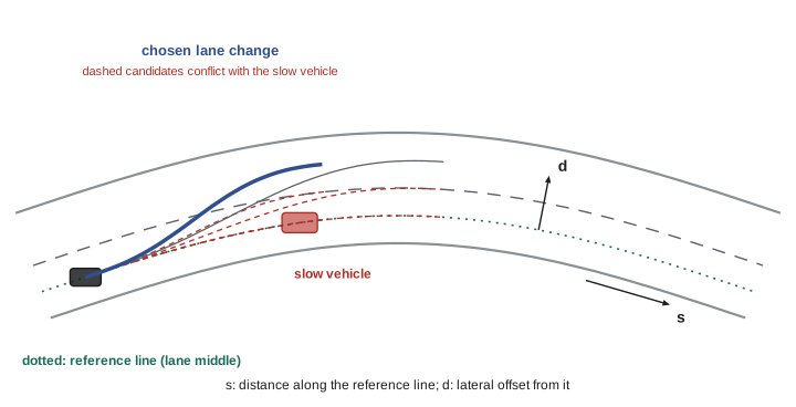
Roads curve, so planning in global x and y coordinates is awkward. Frenet coordinates describe position by \( s \), the distance along a reference line such as the lane centre, and \( d \), the lateral offset from it. A lane change becomes a smooth change in \( d \) while \( s \) increases. A common approach samples many candidate trajectories: for several end times and end offsets, it fits polynomials, typically quintic in \( d \) and quartic in \( s \), that minimize jerk, converts them to global coordinates, checks them against curvature and acceleration limits and against predicted obstacle positions, and picks the lowest-cost survivor. Lattice planners precompute a set of motion primitives on a road-aligned grid and search over them. Optimization-based planners solve directly for a smooth trajectory subject to constraints.

Path tracking: pure pursuit and Stanley

Given a reference path, a tracking controller computes the steering angle. Pure pursuit picks a look-ahead point on the path a distance \( l_d \) ahead and steers along the circular arc that would reach it. With \( \alpha \) the angle between the vehicle heading and the line to the look-ahead point, the bicycle geometry gives:

A longer look-ahead gives smoother but lazier tracking that cuts corners; a shorter one tracks tightly but can oscillate. Look-ahead is usually scaled with speed. The Stanley controller, used by Stanford's vehicle in the 2005 DARPA Grand Challenge, references the front axle and combines heading error \( \psi_e \) with cross-track error \( e \): \( \delta = \psi_e + \arctan(k e / v) \). Both are geometric controllers, simple and robust, and both ignore dynamics, so production systems often add feed-forward from path curvature and use them alongside or inside model predictive control.

# Pure pursuit tracking a straight lane after starting 1.5 m off to the side
import numpy as np
L, v, dt = 2.8, 10.0, 0.02
x, y, th = 0.0, 1.5, 0.0          # start 1.5 m left of the path y = 0
for ld in (5.0, 15.0):            # short and long look-ahead
    x, y, th = 0.0, 1.5, 0.0
    ys = []
    for _ in range(int(8 / dt)):
        gx, gy = x + ld, 0.0      # look-ahead point on the line (approximate)
        alpha = np.arctan2(gy - y, gx - x) - th
        delta = np.arctan2(2 * L * np.sin(alpha), ld)
        delta = np.clip(delta, -0.5, 0.5)
        x += v * np.cos(th) * dt; y += v * np.sin(th) * dt
        th += v / L * np.tan(delta) * dt
        ys.append(y)
    ys = np.array(ys)
    settle = np.argmax(np.abs(ys) < 0.1) * dt
    print(f"look-ahead {ld:4.1f} m: overshoot {max(0, -ys.min()):.2f} m, within 0.1 m after {settle:.2f} s")

look-ahead  5.0 m: overshoot 0.07 m, within 0.1 m after 0.98 s
look-ahead 15.0 m: overshoot 0.07 m, within 0.1 m after 2.96 s

Model predictive control

Model predictive control, MPC, from ROB-310, is the workhorse of advanced vehicle control. At each control step it solves an optimization over a short horizon, typically 1 to 3 seconds, finding the sequence of steering and acceleration inputs that best tracks the reference while respecting limits on steering angle and rate, acceleration, jerk and tire friction, then applies the first input and repeats. MPC handles constraints explicitly, anticipates upcoming curvature and can use a dynamic tire model. Its cost is computation: a nonlinear MPC must solve reliably within tens of milliseconds, every cycle, with a fallback if the solver fails. Longitudinal control, speed tracking and following, is often handled by a separate controller such as adaptive cruise control logic or a longitudinal MPC.

Stopping distance, time to collision and safe following distance

Every planner relies on a few safety quantities. The stopping distance is the distance travelled during the reaction or system latency time \( t_r \) plus the braking distance \( v^2/(2a) \). Time to collision, TTC, is the gap to a lead vehicle divided by the closing speed, assuming both keep their speeds; values below about 2 to 3 s commonly trigger warnings and below about 1.5 s emergency braking. The responsibility-sensitive safety model, RSS, proposed by Mobileye researchers in 2017, formalizes a safe longitudinal distance: the following vehicle must be able to stop without collision even if the lead vehicle brakes as hard as possible, given the follower's response time and its guaranteed braking.

# Stopping distance, time to collision and RSS safe distance on dry and snowy roads
import numpy as np
def stopping(v, tr, a):
    return v * tr + v**2 / (2 * a)
def rss(vr, vf, rho, amax, bmin, bmax):
    d = vr * rho + 0.5 * amax * rho**2 + (vr + rho * amax)**2 / (2 * bmin) - vf**2 / (2 * bmax)
    return max(d, 0.0)
v = 100 / 3.6                                  # 100 km/h in m/s
for surface, mu in (("dry", 0.8), ("snow", 0.3)):
    a = mu * 9.81 * 0.9                        # usable braking
    print(f"{surface:5s}: stop from 100 km/h with 0.5 s latency = {stopping(v, 0.5, a):6.1f} m;"
          f" RSS gap (same speeds) = {rss(v, v, 0.5, 2.0, 0.7*a, a):6.1f} m")
gap, v_ego, v_lead = 40.0, v, 60 / 3.6
ttc = gap / (v_ego - v_lead)
print(f"TTC closing on a 60 km/h car 40 m ahead: {ttc:.2f} s")

dry  : stop from 100 km/h with 0.5 s latency =   68.5 m; RSS gap (same speeds) =   43.3 m
snow : stop from 100 km/h with 0.5 s latency =  159.5 m; RSS gap (same speeds) =   91.8 m
TTC closing on a 60 km/h car 40 m ahead: 3.60 s

# A minimal ROS 2 node that turns a pure pursuit steering command into an Ackermann message
import math
import rclpy
from rclpy.node import Node
from ackermann_msgs.msg import AckermannDriveStamped
from nav_msgs.msg import Odometry

class PurePursuitNode(Node):
    def __init__(self):
        super().__init__('pure_pursuit')
        self.declare_parameter('wheelbase', 2.8)
        self.declare_parameter('lookahead_gain', 0.8)   # look-ahead = gain * speed + 3 m
        self.pub = self.create_publisher(AckermannDriveStamped, '/vehicle/cmd', 10)
        self.create_subscription(Odometry, '/localization/odom', self.on_odom, 10)

    def on_odom(self, msg):
        v = msg.twist.twist.linear.x
        ld = self.get_parameter('lookahead_gain').value * v + 3.0
        alpha = self.angle_to_lookahead_point(msg, ld)     # from the planned path
        L = self.get_parameter('wheelbase').value
        cmd = AckermannDriveStamped()
        cmd.drive.steering_angle = math.atan2(2 * L * math.sin(alpha), ld)
        cmd.drive.speed = self.target_speed()
        self.pub.publish(cmd)

rclpy.init(); rclpy.spin(PurePursuitNode())

In a real stack, the tracking controller is one node among many, subscribing to the localization estimate and planned trajectory and publishing actuator commands at a fixed rate. Parameters such as wheelbase and look-ahead gain are declared so that they can be tuned per vehicle without recompiling, and a watchdog elsewhere checks that commands keep arriving; if they stop, the vehicle brakes to a stop.

Putting the layers together

A typical automated driving stack runs the behaviour planner at a few hertz, the motion planner at 10 to 20 Hz and the tracking controller at 50 to 100 Hz, with actuator loops faster still. Each layer has checks: the motion planner rejects trajectories exceeding friction limits estimated for the current surface, the controller monitors tracking error, and an independent safety monitor can override the stack with a minimal risk manoeuvre if limits are violated. Winter conditions tighten every limit, which is why a vehicle certified for a dry-weather operational design domain must recognize snow and either adapt or exit its ODD.