
ROB-460 · Lesson 10 of 12 · 30 min
Swarms and distributed control
Lesson 9 treated multi-robot teams in which tasks are explicitly allocated, often by a planner or an auction. Swarm robotics takes a different approach: large numbers of relatively simple robots, each using only local sensing and communication, follow simple rules from which useful collective behaviour emerges. No robot knows the whole plan, and no single robot is essential. This lesson covers the principles of swarm robotics, the mathematics of consensus on communication graphs, flocking and formation control, coverage control, stigmergy and threshold-based task allocation, and the difficult questions of designing, verifying and supervising emergent behaviour. It also distinguishes true swarms from centrally choreographed groups, such as most drone light shows.
Principles of swarm robotics
Swarm robotics draws inspiration from social insects, bird flocks and fish schools. An ant colony finds short paths to food, a termite mound regulates its temperature and a flock of starlings turns as one, without any individual directing the group. Researchers identify several properties that swarm systems aim for. Robustness: the loss of some robots degrades performance gradually rather than causing failure. Scalability: the same rules work for ten robots or a thousand, because each robot interacts only with neighbours. Flexibility: the swarm adapts to changes in the environment or task. Simplicity of individuals: each robot can be cheap, with limited sensing, computation and communication.
These properties come with costs. Emergent behaviour can be hard to predict and to design: choosing local rules that produce a desired global outcome is an inverse problem with no general solution. Performance may be lower than with an optimized centralized plan. Verifying that a swarm will never do something unsafe is difficult because the space of possible interactions is enormous. And supervising hundreds of robots requires new forms of human interface. Field applications have so far been more limited than research suggests, but swarm methods are increasingly used for parts of larger systems: distributed sensing, area coverage, formation keeping and resilient communication.
| Approach | Coordination | Typical scale | Strengths | Weaknesses |
|---|---|---|---|---|
| Centralized team | One planner allocates and schedules | A few to tens of robots | Optimal or near-optimal plans | Single point of failure; needs global communication |
| Decentralized team (auctions, consensus) | Robots negotiate explicitly | Tens of robots | Robust, no central planner | Communication overhead grows with team size |
| Swarm | Local rules; emergent behaviour | Tens to thousands | Scalable, robust, simple robots | Hard to design and verify; lower efficiency |
| Choreographed group | Pre-computed trajectories for each robot | Hundreds to thousands (light shows) | Precise visual patterns | Not adaptive; depends on positioning and central timing |
Consensus on communication graphs
Many distributed algorithms reduce to agreement: robots must agree on a heading, a meeting point, a time, or an estimate of a quantity such as average temperature, using only communication with neighbours. Model the robots as nodes of a graph, with an edge between two robots that can communicate. In the simplest consensus protocol, each robot repeatedly moves its value toward the values of its neighbours:
Here \( L = D - A \) is the graph Laplacian, with \( D \) the diagonal matrix of node degrees and \( A \) the adjacency matrix. If the graph is connected and undirected, all values converge to the average of the initial values. The speed of convergence is governed by the second-smallest eigenvalue of \( L \), called the algebraic connectivity \( \lambda_2 \): disagreement decays roughly as \( e^{-\lambda_2 t} \). Well-connected graphs have large \( \lambda_2 \) and agree quickly; long chains and rings of robots, common when robots are strung out along a pipeline or tunnel, have small \( \lambda_2 \) and agree slowly. In discrete time with step size \( \varepsilon \), the update \( x_i \gets x_i + \varepsilon \sum_j (x_j - x_i) \) converges if \( \varepsilon \) is less than one over the maximum degree.
Worked problem
Laplacian of a four-robot chain
Four robots are strung along a tunnel so that each communicates only with its neighbours: 1 to 2, 2 to 3 and 3 to 4. Write the Laplacian and find its algebraic connectivity. The eigenvalues of a path graph with n nodes are \( 2 - 2\cos(k\pi/n) \) for k = 0 to n - 1.
Show solution
- Degrees: 1, 2, 2, 1. Laplacian rows: (1, -1, 0, 0), (-1, 2, -1, 0), (0, -1, 2, -1), (0, 0, -1, 1).
- Eigenvalues: \( 2 - 2\cos(k\pi/4) \) for k = 0, 1, 2, 3, giving 0, 0.586, 2 and 3.414.
- Algebraic connectivity: \( \lambda_2 \approx 0.586 \).
- Disagreement shrinks by a factor \( e \) roughly every \( 1/0.586 \approx 1.7 \) time units.
Answer: The chain has \( \lambda_2 \approx 0.59 \); adding a link between robots 1 and 4 (forming a ring) raises it to 2, speeding agreement by more than three times.
# Discrete-time average consensus on three communication graphs
import numpy as np
rng = np.random.default_rng(10)
n = 20
def laplacian(A):
    return np.diag(A.sum(1)) - A
def chain(n):
    A = np.zeros((n, n))
    for i in range(n - 1): A[i, i + 1] = A[i + 1, i] = 1
    return A
def ring(n):
    A = chain(n); A[0, -1] = A[-1, 0] = 1; return A
def geometric(n, radius):
    while True:
        p = rng.uniform(0, 1, (n, 2))
        A = ((np.linalg.norm(p[:, None] - p[None], axis=2) < radius) & ~np.eye(n, dtype=bool)).astype(float)
        if np.linalg.eigvalsh(laplacian(A))[1] > 1e-9: return A     # keep only connected graphs
x0 = rng.uniform(0, 100, n)          # e.g. each robot's local temperature estimate
for name, A in [("chain", chain(n)), ("ring", ring(n)), ("random geometric", geometric(n, 0.4))]:
    L = laplacian(A); lam2 = np.linalg.eigvalsh(L)[1]
    eps = 0.9 / A.sum(1).max()
    x, k = x0.copy(), 0
    while np.ptp(x) > 0.01 * np.ptp(x0):
        x = x - eps * L @ x; k += 1
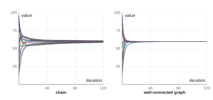
print(f"{name:17s} lambda2 = {lam2:6.3f} steps to 1 % disagreement: {k:5d} average kept: {x.mean():.3f} vs {x0.mean():.3f}")chain lambda2 = 0.025 steps to 1 % disagreement: 220 average kept: 59.465 vs 59.465 ring lambda2 = 0.098 steps to 1 % disagreement: 72 average kept: 59.465 vs 59.465 random geometric lambda2 = 0.935 steps to 1 % disagreement: 27 average kept: 59.465 vs 59.465
The chain of twenty robots needs about eight times as many iterations to agree as the well-connected random network, and closing the chain into a ring with one extra link makes agreement about three times faster. In every case the average is preserved, which is what makes consensus useful for distributed estimation: robots can compute the average of their measurements without sending them all to one place. Practical versions must handle changing graphs as robots move, communication delays, packet loss and robots that fail or report faulty values; resilient consensus algorithms discard extreme values from neighbours so that a few faulty or malicious robots cannot pull the group arbitrarily.
Flocking and formations
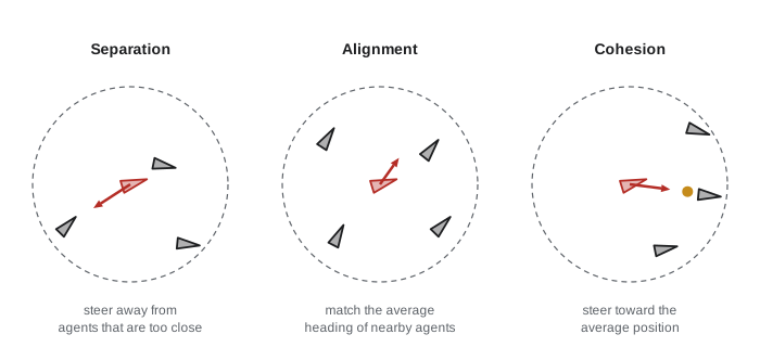
In 1987 Craig Reynolds showed that realistic animated flocks, which he called boids, emerge when each agent follows three local rules: separation (steer away from neighbours that are too close), alignment (steer toward the average heading of neighbours) and cohesion (steer toward the average position of neighbours). Later work, notably by Olfati-Saber, gave flocking algorithms with proofs of collision avoidance and velocity matching for robots, using potential functions for spacing and consensus for alignment. Flocking is used for groups of drones or surface vessels moving together without fixed positions.
# A minimal boids simulation: does the group align and stay together?
import numpy as np
rng = np.random.default_rng(3)
N, R, dt, vmax = 40, 15.0, 0.1, 5.0
pos = rng.uniform(0, 60, (N, 2)); vel = rng.normal(0, 2, (N, 2))
def step(pos, vel, w_sep=1.5, w_ali=1.0, w_coh=0.4):
    d = pos[:, None, :] - pos[None, :, :]
    dist = np.linalg.norm(d, axis=2) + np.eye(N) * 1e9
    nb = dist < R
    acc = np.zeros_like(vel)
    for i in range(N):
        if nb[i].any():
            close = dist[i] < 4.0
            acc[i] += w_sep * (d[i][close] / dist[i][close, None] ** 2).sum(0) if close.any() else 0
            acc[i] += w_ali * (vel[nb[i]].mean(0) - vel[i])
            acc[i] += w_coh * (pos[nb[i]].mean(0) - pos[i]) * 0.1
    vel = vel + acc * dt
    speed = np.linalg.norm(vel, axis=1, keepdims=True)
    vel = np.where(speed > vmax, vel / speed * vmax, vel)
    return pos + vel * dt, vel
def order(vel):                        # 1.0 means all agents move in the same direction
    u = vel / np.linalg.norm(vel, axis=1, keepdims=True)
    return np.linalg.norm(u.mean(0))
for t in range(0, 601):
    if t % 150 == 0:
        dmin = (np.linalg.norm(pos[:, None] - pos[None], axis=2) + np.eye(N) * 1e9).min()
        print(f"step {t:3d}: alignment order {order(vel):.2f}, closest pair {dmin:5.2f} m, group spread {pos.std(0).mean():5.1f} m")
pos, vel = step(pos, vel)step 0: alignment order 0.02, closest pair 0.14 m, group spread 16.9 m step 150: alignment order 0.18, closest pair 3.44 m, group spread 11.9 m step 300: alignment order 0.27, closest pair 2.82 m, group spread 7.8 m step 450: alignment order 0.61, closest pair 2.19 m, group spread 6.6 m step 600: alignment order 0.95, closest pair 2.07 m, group spread 6.3 m
The order parameter rises as the agents align, and separation keeps them from colliding, without any agent knowing the group's overall direction. Changing the weights changes the behaviour: too little cohesion and the flock splits; too much and it collapses into a tight cluster. Tuning such parameters for robust behaviour across many conditions is a central challenge of swarm design, and automatic design methods such as evolutionary algorithms and reinforcement learning are often used to search for good local rules.
Formation control asks robots to hold a specific geometric shape, such as a line of AUVs spaced 200 m apart to survey with side-scan sonar, or a triangle of drones for stereo imaging. Displacement-based formation control applies consensus to the differences between actual and desired relative positions, so the formation can translate while keeping its shape; distance-based methods use only measured distances, which avoids the need for a shared coordinate frame but needs rigid graph structures to define a unique shape. Leader-follower schemes are simpler but depend on the leader.
Coverage, stigmergy and division of labour
Coverage control distributes robots over an area to monitor it well. In the method of Cortés and colleagues, each robot is responsible for its Voronoi cell, the set of points closer to it than to any other robot, and moves toward the centroid of its cell weighted by a density function describing where coverage matters most. Repeating this, a form of Lloyd's algorithm, converges to a centroidal Voronoi configuration that locally optimizes coverage, using only information about neighbours. The approach suits sensor networks of drones or surface vessels monitoring an oil spill, an algal bloom or a wildfire perimeter, and the density function can be updated as new measurements arrive.
Stigmergy is coordination through changes in the environment: ants lay pheromone trails that others follow, reinforcing short paths. Robots can use virtual pheromones in a shared map, marks such as RFID tags or simply the state of the work itself, for example a weeding robot avoiding rows that look recently treated. Division of labour in insect colonies is often explained by response thresholds: each individual takes up a task when a stimulus, such as the amount of unfinished work, exceeds its personal threshold, and thresholds vary across individuals. Robots using randomized thresholds can divide work among tasks in proportion to demand without explicit negotiation, adapting as demand changes and as robots fail.
Worked problem
Response-threshold task switching
A swarm uses the response function \( P = s^2/(s^2 + \theta^2) \) for the probability that a robot starts a task with stimulus s, where \( \theta \) is the robot's threshold. For a robot with \( \theta = 10 \), compute P when the stimulus is 5, 10 and 20.
Show solution
- s = 5: \( 25 / (25 + 100) = 0.20 \).
- s = 10: \( 100 / 200 = 0.50 \).
- s = 20: \( 400 / 500 = 0.80 \).
Answer: The probability rises from 0.2 to 0.5 to 0.8 as the stimulus grows; robots with lower thresholds join earlier, so the number of robots on a task tracks the amount of work waiting.
Swarms in practice
Research swarms demonstrate scale. Harvard's Kilobot project showed in 2014 that 1,024 small, inexpensive robots could self-assemble into shapes using only local infrared communication. Drone light shows with thousands of drones are visually swarm-like, but they are usually choreographed: each drone follows a pre-computed trajectory using RTK positioning and synchronized timing, with a central ground station; they show the value of precise positioning and fleet management rather than emergent behaviour. Field uses of swarm ideas include distributed ocean sensing with many floats and gliders, cooperative search with drones, and formations of surface vessels for survey. Militaries in several countries are investing heavily in drone swarms and in countering them; ROB-450 lesson 11 discussed the ethical and legal debate about autonomy in the use of force, which applies with particular force to swarms because human control over each robot's actions may be weak.
| Design concern | Why it matters for swarms | Approaches |
|---|---|---|
| Emergent failure modes | Local rules can produce unexpected global behaviour such as oscillation or clustering | Simulation over many scenarios, formal methods for simplified models, staged field trials |
| Faulty or malicious robots | A few bad robots can mislead neighbours | Resilient consensus, outlier rejection, authentication |
| Communication limits | Range, interference and congestion grow with numbers | Local, low-bandwidth messages; stigmergy; event-triggered communication |
| Human supervision | Operators cannot control hundreds of robots individually | Commands at swarm level (areas, densities, behaviours), summary displays, playbooks |
| Recovery and environmental impact | Lost robots may become litter or hazards | Biodegradable or recoverable designs, tracking, accounting for every unit |
Human-swarm interaction is an active research area. Operators of large swarms work best with high-level commands such as setting the area to cover, the density of robots, or the behaviour to adopt, and with displays that summarize the swarm's state rather than showing every robot. The same principles apply to supervising fleets of field robots, as lesson 11 develops.
Common mistakes
MistakeCalling any large group of robots a swarm.
InsteadDistinguish emergent, locally controlled swarms from centrally planned teams and choreographed groups such as light shows.
MistakeAssuming consensus will be fast because each update is simple.
InsteadConvergence depends on algebraic connectivity; chains and sparse graphs agree slowly, so check \( \lambda_2 \) for the expected topology.
MistakeTuning swarm rules in one simulation scenario.
InsteadTest across many initial conditions, densities, failures and disturbances to find emergent failure modes.
MistakeTrusting every neighbour's value in distributed estimation.
InsteadUse resilient consensus that discards extreme values, so faulty or malicious robots cannot dominate.
MistakeGiving a swarm operator control of individual robots.
InsteadProvide swarm-level commands and summary displays suited to many robots.
Summary and key terms
- Swarm robotics uses many simple robots following local rules to achieve robust, scalable collective behaviour.
- Average consensus with the graph Laplacian lets robots agree using only neighbours, at a rate set by the algebraic connectivity.
- Reynolds' separation, alignment and cohesion rules produce flocking; formal flocking algorithms add guarantees.
- Formation control uses consensus on relative positions or distances to hold shapes such as survey lines.
- Voronoi-based coverage control distributes robots according to a density of importance using only local information.
- Stigmergy and response thresholds coordinate work through the environment and simple individual rules.
- Design, verification, fault tolerance and human supervision are the main barriers to field swarms.
- Swarm robotics
- The study of large groups of simple robots whose collective behaviour emerges from local interactions.
- Emergence
- Global behaviour arising from local interactions without central control.
- Graph Laplacian
- The matrix L = D - A describing a communication graph, used in consensus analysis.
- Algebraic connectivity
- The second-smallest eigenvalue of the graph Laplacian, measuring how well connected the graph is.
- Average consensus
- A distributed protocol in which all agents converge to the average of their initial values.
- Boids
- Reynolds' model of flocking agents following separation, alignment and cohesion rules.
- Formation control
- Controlling a group of robots to achieve and maintain a desired geometric arrangement.
- Voronoi cell
- The region of points closer to one robot than to any other.
- Stigmergy
- Indirect coordination through modifications of the shared environment.
- Response threshold
- A level of task stimulus above which an individual becomes likely to take up the task.
Practice problems
Work each problem on paper first, then reveal the answer to check.
Name three properties that swarm robotics aims for.
Show answer
Robustness, scalability, flexibility (and simplicity of individuals).
Write the Laplacian for three robots all connected to each other.
Show answer
Rows (2, -1, -1), (-1, 2, -1), (-1, -1, 2).
What is the algebraic connectivity of the fully connected three-robot graph?
Show answer
Its eigenvalues are 0, 3, 3, so \( \lambda_2 = 3 \).
Why does average consensus preserve the average of initial values on an undirected graph?
Show answer
The Laplacian's rows and columns sum to zero, so the sum of all values does not change.
What condition on step size ensures discrete-time consensus converges?
Show answer
The step size must be less than one over the maximum node degree (for this simple update).
State Reynolds' three flocking rules.
Show answer
Separation, alignment and cohesion.
What happens to a flock if cohesion is too weak?
Show answer
It tends to split into separate groups.
How does Voronoi coverage control use only local information?
Show answer
Each robot needs only its neighbours' positions to compute its Voronoi cell and move toward the cell's weighted centroid.
With \( P = s^2/(s^2+\theta^2) \) and \( \theta = 4 \), what is P at s = 4?
Show answer
0.5.
Why are most drone light shows not true swarms?
Show answer
Each drone follows a pre-computed trajectory with central timing and positioning, rather than behaviour emerging from local rules.
Lesson quiz · 5 questions
Score 60% or more to complete this lesson.
Create a free account to save your progress, take quizzes and earn a certificate.