
PHOT-420 · Lesson 4 of 12 · 29 min
HDR imaging and tone mapping
A sunlit landscape with deep shade, a backlit portrait by a window and a night street with bright signs all contain a wider range of brightness than a single exposure can record or a screen can display. High dynamic range (HDR) imaging solves the first problem by combining information from several exposures, or from many underexposed frames, into one image with far more tonal range. Tone mapping solves the second by compressing that range into something a display or print can show while keeping the scene looking natural, or deliberately stylized. This lesson measures dynamic range in stops, merges bracketed exposures into a radiance map with weighted averaging, applies the Reinhard tone curve, and explains local tone mapping, exposure fusion and the new generation of HDR displays and gain-map files that let a photo show bright highlights on capable screens.
Dynamic range in stops
Dynamic range is the ratio between the brightest and darkest values that can be recorded or shown with acceptable quality. Photographers measure it in stops, where each stop is a doubling:
A sunlit scene with deep shadows can exceed 14 to 17 stops. A single phone frame might capture around 10 to 12 usable stops, a large-sensor camera 12 to 15 at base ISO, a standard display about 8 to 10 stops of contrast in practice, and a matte print about 6 to 7 stops. These figures are approximate, depend on how "acceptable" noise is defined, and vary between devices. The mismatch at each stage, scene to sensor and sensor to display, is the reason for HDR capture and tone mapping.
Worked problem
Dynamic range of a scene
A light meter reads a sunlit white wall at 16,000 cd/m² and a shaded doorway interior at 4 cd/m². How many stops is this, and can a sensor with 12 stops record both with detail?
Show solution
- Ratio: \( 16\,000 / 4 = 4000 \).
- Stops: \( \log_2 4000 \approx 11.97 \), about 12 stops.
- The scene uses almost all of a 12-stop sensor's range, leaving the darkest tones near the noise floor.
Answer: About 12 stops; a single exposure can just hold both, but the doorway will be noisy, so an HDR merge would improve it.
| Stage | Typical range | Notes |
|---|---|---|
| Bright outdoor scene with shade | 14 to 17+ stops | Includes sun-lit and deep-shadow surfaces |
| Single phone frame | 10 to 12 stops | Small pixels limit full-well capacity |
| Large-sensor camera at base ISO | 12 to 15 stops | Falls as ISO rises |
| Standard dynamic range display | About 8 to 10 stops | Depends on panel and ambient light |
| HDR display (peak 1,000+ nits) | 12+ stops | Bright highlights above diffuse white |
| Matte print | About 6 to 7 stops | Paper white versus maximum black ink |
Merging brackets into a radiance map
The classic approach, developed by Paul Debevec and Jitendra Malik and by others in the 1990s, takes several exposures at different shutter speeds. After converting each to linear values (raw data is already linear; JPEGs must be linearized by inverting the camera response curve), each pixel value is divided by its exposure time to estimate scene radiance. The estimates from different frames are combined with weights that favor well-exposed values and ignore clipped or very dark ones:
Here \( z_k \) is the linear pixel value in frame \( k \), \( t_k \) its exposure time and \( w \) a weighting function that is zero for clipped values and small near black. A common choice is a "hat" function peaking at mid-tones. Better weightings use the noise model: since a frame with a longer exposure has a higher SNR for the same radiance, it should get more weight unless it is clipped. The result is a floating-point radiance map with far more range than any one frame.
import numpy as np
rng = np.random.default_rng(420)
E = np.logspace(-3, 1.2, 2000)                 # scene radiance spanning about 14 stops
times = [1 / 1000, 1 / 125, 1 / 15]            # three brackets, 3 stops apart
full = 1.0                                      # sensor saturation
def capture(t):
    signal = E * t * 600                        # arbitrary sensitivity
    noisy = signal + rng.normal(0, np.sqrt(0.002 * signal + 1e-5))
    return np.clip(noisy, 0, full)
frames = [capture(t) for t in times]
num = np.zeros_like(E); den = np.zeros_like(E)
for z, t in zip(frames, times):
    w = np.where(z >= 0.98 * full, 0.0, z * t)  # zero weight if clipped; prefer long exposures (higher SNR)
    num += w * z / (t * 600); den += w
merged = num / np.maximum(den, 1e-12)
for z, t in zip(frames, times):
    ok = (z > 0.01) & (z < 0.98)
    print(f"1/{round(1 / t):4d} s: usable for {ok.mean() * 100:4.1f} % of radiances")
rel = np.abs(merged - E) / E
print(f"merged map: median relative error {np.median(rel) * 100:.1f} %, usable range {np.log2(E.max() / E.min()):.1f} stops")1/1000 s: usable for 48.1 % of radiances 1/ 125 s: usable for 47.5 % of radiances 1/ 15 s: usable for 33.1 % of radiances merged map: median relative error 7.8 %, usable range 14.0 stops
Each bracket alone is usable for only part of the radiance range, but the merged map covers all of it, with a modest median error that is largest in the deepest shadows, where even the longest frame collects few photons. The long exposure handles shadows, the short exposure handles highlights, and the weights blend smoothly between them.
Ghosts, alignment and burst HDR
Brackets have a weakness: frames at different exposures look different, which makes alignment harder, and moving subjects appear at different positions in frames that dominate different tones, causing ghosts. Phones therefore increasingly use the burst approach from lesson 3: many identical underexposed frames, aligned and robustly merged, with the shadows lifted in tone mapping. The merged result's improved SNR in the shadows effectively extends dynamic range downward. Some pipelines add one or two longer frames to boost shadow quality, and some sensors capture multiple exposures in a single readout using dual conversion gain or staggered exposures, reducing the time gap between them and therefore ghosting. On dedicated cameras, handheld bracketing with in-camera or software merging remains common, and good HDR software includes deghosting that picks one frame for areas with motion.
Global tone mapping
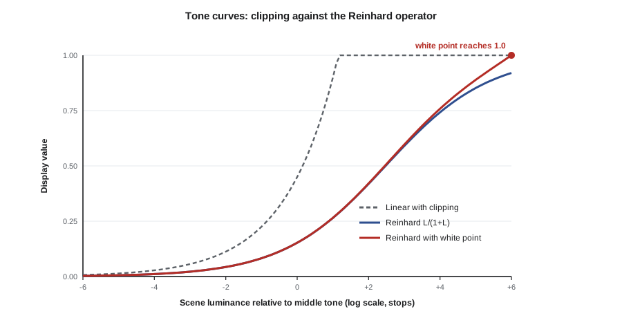
A radiance map cannot be displayed directly: its values span thousands to one, while a display spans perhaps a few hundred to one in practice. Tone mapping compresses the range. A global operator applies the same curve to every pixel based only on its value. Erik Reinhard and colleagues proposed a widely used simple operator in 2002. After scaling the image so that its log-average luminance maps to a chosen middle gray, each luminance \( L \) is compressed by:
Dark values (\( L \ll 1 \)) pass almost unchanged, while bright values approach 1 asymptotically, so highlights are compressed but never clip. An extended version adds a white point \( L_w \), the smallest luminance that maps to pure white:
Global curves are fast and preserve the overall order of brightness, but compressing a large range globally reduces local contrast, making images look flat. Filmic curves used in games and some raw converters add an S-shaped toe and shoulder to imitate film's response.
import numpy as np
L = 0.18 * 2.0 ** np.arange(-6, 7, 2)              # scene luminances from -6 to +6 stops around mid-tone
key = 0.18
Ls = L / 0.18 * key                                 # already keyed to the mid-tone
simple = Ls / (1 + Ls)
Lw = Ls.max()
ext = Ls * (1 + Ls / Lw ** 2) / (1 + Ls)
for l, a, b in zip(L, simple, ext):
    print(f"scene {l:8.4f} -> simple {a:.3f}  with white point {b:.3f}")
print(f"contrast ratio in: {L.max() / L.min():.0f}:1, out (white point): {ext.max() / ext.min():.0f}:1")scene 0.0028 -> simple 0.003 with white point 0.003 scene 0.0112 -> simple 0.011 with white point 0.011 scene 0.0450 -> simple 0.043 with white point 0.043 scene 0.1800 -> simple 0.153 with white point 0.153 scene 0.7200 -> simple 0.419 with white point 0.421 scene 2.8800 -> simple 0.742 with white point 0.758 scene 11.5200 -> simple 0.920 with white point 1.000 contrast ratio in: 4096:1, out (white point): 357:1
The output shows the compression: a 4,096:1 scene range is squeezed into a few hundred to one, with the brightest value reaching exactly 1.0 when a white point is used. Shadows keep roughly their relative steps, while each stop of highlight occupies less and less of the output range.
Local tone mapping and exposure fusion
Local operators let the curve vary across the image, so a dark interior and a bright window can each keep good contrast. The simplest idea is to separate an image into a smooth base layer containing large-scale brightness and a detail layer containing texture, compress only the base, and add the detail back. Using an ordinary blur to find the base creates halos, bright or dark fringes along strong edges, because the blur crosses the edge. Edge-preserving filters such as the bilateral filter, guided filter and local Laplacian filters avoid this. The over-processed "HDR look" of the late 2000s, with glowing halos and gray skies, came from aggressive local operators.
Exposure fusion, introduced by Tom Mertens, Jan Kautz and Frank Van Reeth in 2007, skips the radiance map altogether. It blends the differently exposed frames directly, weighting each pixel by contrast, saturation and well-exposedness, and blends them across a Laplacian pyramid so that transitions are smooth at every scale. The result looks natural and needs no tone curve. Many phone pipelines use ideas from exposure fusion: Google's HDR+ described synthesizing a short and a long "virtual exposure" from the merged burst and fusing them. Today, neural networks often predict local tone curves or adjustment grids from a low-resolution version of the image, an approach known from research on deep bilateral learning, then apply them at full resolution quickly.
Semantic tone mapping and the phone look
Modern phones adjust tone by content. Face detection keeps skin at a pleasing brightness; sky segmentation darkens and saturates skies; and different rules apply to foliage, food or text. This semantic processing is why many phone photos look bright and evenly lit, with shadows lifted and highlights held, sometimes described as flat or "HDR-ish". Critics argue that it removes the drama of light and shadow; manufacturers have responded with styles and more natural options. For professional work, choosing computational raw or a natural style and doing your own tone mapping keeps the creative decisions yours.
| Approach | How it works | Strength | Risk |
|---|---|---|---|
| Global curve (Reinhard, filmic) | Same curve for all pixels | Fast, no halos | Flat local contrast |
| Base-detail with edge-aware filter | Compress base layer, keep detail | Good local contrast | Halos if filter is poor |
| Exposure fusion | Blend frames by quality weights | Natural, no radiance map | Limited extreme range |
| Learned local curves | Network predicts adjustments | Fast, content-aware | Training bias, consistent look |
| Semantic adjustments | Rules per segmented region | Pleasing faces and skies | Uniform, less dramatic light |
HDR display and gain maps
For most of digital photography's history, the final image was standard dynamic range (SDR): diffuse white was the brightest the display could show. HDR displays, now common on phones, laptops and televisions, can show highlights several times brighter than diffuse white. Video has HDR standards such as HDR10, HLG and Dolby Vision. For still photos, the industry converged on gain maps: a file stores a normal SDR image plus a secondary map recording how much brighter each region should be on an HDR display. Viewers that do not understand the gain map show the SDR image normally; capable viewers apply the map. The ISO 21496-1 standard for gain maps, published in 2025, aims to unify earlier formats such as Google's Ultra HDR JPEG and Apple's adaptive HDR approach, and Adobe and others support gain maps in editing and export (status at the time of writing; check software support). This changes tone mapping: rather than compressing everything into SDR, the pipeline can keep bright specular highlights and sunsets genuinely bright on screens that can show them.
Worked problem
Headroom on an HDR display
A phone display shows diffuse white at 400 nits and can reach 1,600 nits peak for highlights. How many stops of headroom above diffuse white is that?
Show solution
- Ratio: \( 1600 / 400 = 4 \).
- Stops: \( \log_2 4 = 2 \).
Answer: Two stops of headroom; a gain map can make highlights up to four times brighter than paper-white on this display.
For photographers delivering work, HDR output raises new questions: clients viewing on SDR screens see the base image; print cannot reproduce the headroom; and social platforms handle gain maps inconsistently. Proof both versions and keep the SDR rendition strong on its own.
Common mistakes
MistakeMerging JPEG brackets without linearizing them
InsteadConvert to linear values (or use raw files) before dividing by exposure time and averaging.
MistakeGiving clipped pixels weight in the merge
InsteadSet weights to zero for clipped values so they do not drag the radiance estimate down.
MistakeUsing strong local tone mapping with simple blurs
InsteadUse edge-preserving filters and moderate strength to avoid halos.
MistakeAssuming everyone sees the HDR highlights you see
InsteadCheck the SDR base image and proof on standard screens and in print.
MistakeIgnoring motion when bracketing
InsteadUse deghosting, burst HDR or a single exposure when subjects move.
Summary and key terms
- Dynamic range is measured in stops as \( \log_2(L_{\max}/L_{\min}) \), and scenes often exceed both sensors and displays.
- Bracket merging divides linear values by exposure time and averages with weights that exclude clipped and noisy values.
- Burst HDR uses identical underexposed frames to avoid alignment and ghosting problems.
- Global operators such as Reinhard's \( L/(1+L) \) compress highlights smoothly but reduce local contrast.
- Local tone mapping and exposure fusion preserve local contrast; poor filters create halos.
- Phones apply semantic tone mapping to faces, skies and other regions.
- Gain maps (ISO 21496-1) store extra highlight brightness for HDR displays alongside an SDR base image.
- Dynamic range
- The ratio between the brightest and darkest usable values, usually in stops.
- Bracketing
- Taking several exposures at different settings of the same scene.
- Radiance map
- A floating-point image estimating relative scene radiance from merged exposures.
- Camera response curve
- The function mapping scene exposure to recorded pixel values, inverted to linearize JPEGs.
- Tone mapping
- Compressing a high dynamic range image into a range a display or print can show.
- Reinhard operator
- A global tone curve \( L/(1+L) \), optionally with a white point.
- Halo
- A bright or dark fringe along a strong edge caused by local tone mapping.
- Exposure fusion
- Blending differently exposed frames directly using quality weights and pyramids.
- Gain map
- An auxiliary image recording how much brighter regions should appear on an HDR display.
- Headroom
- The brightness available above diffuse white on an HDR display.
Practice problems
Work each problem on paper first, then reveal the answer to check.
A scene ranges from 2 to 8,192 cd/m². How many stops?
Show answer
\( \log_2 4096 = 12 \) stops.
Why are clipped pixels given zero weight in an HDR merge?
Show answer
Their true value is unknown, so including them would underestimate radiance.
A linear pixel value of 0.4 was recorded at 1/100 s. What radiance estimate does it give in relative units?
Show answer
\( 0.4 / 0.01 = 40 \).
Apply the simple Reinhard operator to \( L = 3 \).
Show answer
\( 3/4 = 0.75 \).
What causes halos in local tone mapping?
Show answer
Blurring across strong edges when separating base and detail layers.
How does exposure fusion differ from radiance-map HDR?
Show answer
It blends frames directly by quality weights without building a radiance map or tone curve.
Why do burst HDR pipelines produce fewer ghosts than brackets?
Show answer
Identical frames align easily and robust merging rejects moving pixels.
A display has diffuse white at 500 nits and peak 2,000 nits. How many stops of headroom?
Show answer
Two stops.
What does a viewer that ignores gain maps display?
Show answer
The standard dynamic range base image.
Give one reason to shoot computational raw for professional work.
Show answer
To make your own tone and color decisions instead of accepting semantic phone processing.
Lesson quiz · 5 questions
Score 60% or more to complete this lesson.
Create a free account to save your progress, take quizzes and earn a certificate.