
PHOT-420 · Lesson 8 of 12 · 28 min
AI denoising, sharpening and upscaling
Some of the most useful AI tools in photography do not create new scenes; they clean up and enlarge the ones you captured. Since about 2020, raw converters and standalone applications have offered neural network denoising that turns high-ISO files from unusable to printable, deblurring that rescues slightly soft shots, and upscaling that enlarges a small file for a large print. These tools are trained on millions of image pairs and can be astonishingly good, but they work by predicting what a clean image probably looked like. This lesson compares classical and learned denoising, explains sharpening from unsharp masking to deconvolution and learned deblurring, introduces image quality metrics such as PSNR and SSIM, and examines the perception-distortion trade-off that explains why the most pleasing result is not always the most faithful one. PHOT-202 covered how to use noise reduction and sharpening controls in editing; this lesson explains what happens underneath.
Classical denoising
Denoising tries to remove random variation while keeping real detail. The simplest approach, Gaussian blurring, averages each pixel with its neighbors weighted by distance. It reduces noise effectively but blurs edges and texture equally, because it cannot tell noise from detail. The bilateral filter, introduced by Carlo Tomasi and Roberto Manduchi in 1998, adds a second weight based on similarity of brightness: neighbors with very different values, such as those across an edge, contribute little. Edges are preserved, but fine textures similar in contrast to the noise are still smoothed, and strong settings produce a cartoon-like look.
Non-local means, introduced by Antoni Buades and colleagues in 2005, goes further: it averages each pixel with others anywhere in the image whose surrounding patches look similar, exploiting the repetition found in natural images. BM3D (block-matching and 3D filtering, 2007) groups similar patches into stacks and filters them jointly in a transform domain; for over a decade it was the benchmark that new methods had to beat. All of these methods rely on hand-designed assumptions about what images look like.
import numpy as np
rng = np.random.default_rng(420)
h, w = 64, 64
clean = np.zeros((h, w)); clean[:, 32:] = 1.0             # a sharp step edge
clean = 0.2 + 0.6 * clean
noisy = clean + rng.normal(0, 0.08, clean.shape)
def shifted(img, r):
    p = np.pad(img, r, mode="reflect")
    for dy in range(-r, r + 1):
        for dx in range(-r, r + 1):
            yield dy, dx, p[r + dy:r + dy + h, r + dx:r + dx + w]
def gaussian(img, r=3, s=1.5):
    num = np.zeros_like(img); den = 0
    for dy, dx, sh in shifted(img, r):
        g = np.exp(-(dy * dy + dx * dx) / (2 * s * s)); num += g * sh; den += g
    return num / den
def bilateral(img, r=3, s=1.5, sr=0.15):
    num = np.zeros_like(img); den = np.zeros_like(img)
    for dy, dx, sh in shifted(img, r):
        g = np.exp(-(dy * dy + dx * dx) / (2 * s * s)) * np.exp(-((sh - img) ** 2) / (2 * sr * sr))
        num += g * sh; den += g
    return num / den
def psnr(a, b): return 10 * np.log10(1.0 / np.mean((a - b) ** 2))
for name, out in [("noisy", noisy), ("gaussian", gaussian(noisy)), ("bilateral", bilateral(noisy))]:
    flat = out[:, 4:24].std()
    edge = out[:, 33].mean() - out[:, 30].mean()       # contrast 3 px across the edge
print(f"{name:9s} PSNR {psnr(out, clean):5.1f} dB flat noise {flat:.3f} edge contrast {edge:.2f} (true 0.60)")noisy PSNR 22.1 dB flat noise 0.079 edge contrast 0.58 (true 0.60) gaussian PSNR 26.9 dB flat noise 0.014 edge contrast 0.42 (true 0.60) bilateral PSNR 31.3 dB flat noise 0.026 edge contrast 0.59 (true 0.60)
Both filters cut noise in flat areas substantially, but the Gaussian blur smears the edge, cutting contrast across it, while the bilateral filter keeps the edge almost intact and earns a higher peak signal-to-noise ratio (PSNR). Real images have textures as well as edges, and there the bilateral filter also struggles, which is where learned methods excel.
Learned denoising
A denoising neural network is trained on pairs of noisy and clean images. Clean targets come from long exposures, averages of many frames or synthetic noise added to clean images using the noise model from lesson 2. A convolutional network such as DnCNN (2017) learns to predict the noise, or the clean image, from the noisy input. Because it has seen millions of examples, it learns what fur, foliage, skin and fabric look like and preserves them far better than hand-designed filters. Networks that operate on raw data before demosaicing do better still, because noise is simpler there and has not yet been spread and correlated by demosaicing and color correction. Adobe's AI Denoise (2023), DxO's DeepPRIME and similar tools from other companies work on raw files for this reason, often combining denoising with demosaicing in one network (vendor descriptions; implementation details are proprietary).
Learned denoisers can produce results that look like a camera two or three stops better. Their failure modes are characteristic: at extreme noise levels they may invent texture, turning noise into plausible-looking but false detail such as feathers or brickwork; they may smooth unusual textures they have not been trained on; and results can vary between software versions. Photographers should inspect critical areas at 100 percent and compare with the original, especially for scientific, forensic or documentary images.
| Method | Key idea | Strength | Weakness |
|---|---|---|---|
| Gaussian blur | Average nearby pixels | Fast, simple | Blurs all detail |
| Bilateral filter | Weight by distance and similarity | Preserves strong edges | Smooths fine texture, cartoon look |
| Non-local means | Average similar patches anywhere | Preserves repeated texture | Slow, artifacts at high noise |
| BM3D | Filter stacks of similar patches jointly | Strong classical benchmark | Slow, hand-tuned |
| Learned (CNN or transformer) | Trained on noisy and clean pairs | Best detail at high ISO | May invent texture, version-dependent |
Sharpening and deblurring
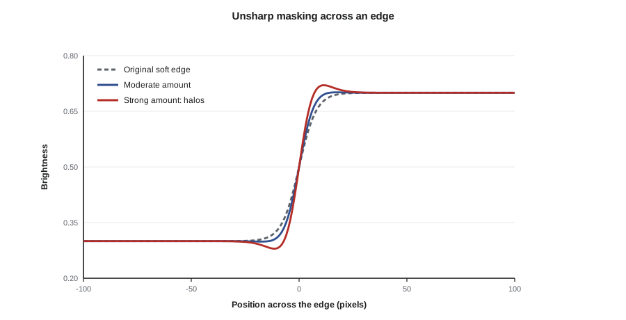
Sharpening increases the contrast of edges and fine detail. The classic unsharp mask, borrowed from darkroom technique, subtracts a blurred copy of the image from the original to isolate detail, then adds a scaled amount of that detail back:
Here \( G_\sigma * I \) is the image blurred with a Gaussian of radius \( \sigma \) and \( \alpha \) is the amount. Unsharp masking adds overshoot at edges, which looks crisp at moderate settings and creates visible halos at strong ones. It also amplifies noise, which is why sharpening is usually masked to edges.
Deconvolution attempts to undo a known blur. If the blur is described by a point spread function (PSF), such as lens blur, defocus or a motion path, deconvolution estimates the original image that, when blurred by that PSF, gives the observed one. Classical methods include Wiener deconvolution and the iterative Richardson-Lucy algorithm, used in astronomy and microscopy. Deconvolution is ill-posed: noise is amplified at frequencies the blur suppressed, so regularization is required. Learned deblurring networks, trained on sharp images blurred synthetically, can remove motion blur and missed focus to a degree that seemed impossible a decade ago, but heavy blur destroys information, and what returns is partly a prediction.
import numpy as np
rng = np.random.default_rng(420)
x = np.linspace(-1, 1, 400)
edge = 0.3 + 0.4 / (1 + np.exp(-x * 25))              # a soft edge from 0.3 to 0.7
noisy = edge + rng.normal(0, 0.01, x.size)
def blur(v, s=6):
    k = np.exp(-0.5 * (np.arange(-20, 21) / s) ** 2); k /= k.sum()
    return np.convolve(np.pad(v, 20, mode="edge"), k, mode="valid")
for amount in (0.0, 0.5, 1.0, 2.0):
    out = noisy + amount * (noisy - blur(noisy))
    slope = np.max(np.gradient(out[190:210]))
    overshoot = out.max() - 0.7
    noise = out[:100].std()
print(f"amount {amount:.1f}: max edge slope {slope:.4f} overshoot {overshoot:+.3f} flat noise {noise:.4f}")amount 0.0: max edge slope 0.0228 overshoot +0.027 flat noise 0.0081 amount 0.5: max edge slope 0.0287 overshoot +0.040 flat noise 0.0120 amount 1.0: max edge slope 0.0345 overshoot +0.052 flat noise 0.0159 amount 2.0: max edge slope 0.0462 overshoot +0.077 flat noise 0.0237
As the amount increases, the edge gets steeper, but overshoot (the halo) grows and noise in flat areas rises. Good sharpening balances these, and modern raw converters apply learned or edge-aware sharpening that avoids amplifying noise in smooth areas.
Upscaling
Upscaling enlarges an image to more pixels. Classical interpolation (nearest neighbor, bilinear, bicubic, Lanczos) estimates new pixels from smooth functions of their neighbors; the result is larger but soft, because no new detail is added. Learned single-image super-resolution, starting with SRCNN in 2014 and advancing through generative adversarial networks such as ESRGAN (2018) and diffusion-based upscalers, predicts high-resolution detail from training on pairs of downsampled and original images. These models produce sharp textures, crisp hair and readable-looking text, but much of this detail is invented: the network has learned what high-resolution images typically look like and generates something consistent with the low-resolution input. Unlike multi-frame super-resolution (lesson 7), no new measurements are involved.
Upscalers are valuable for print enlargements, restoring old low-resolution files, and preparing images for large displays. They are inappropriate where the detail itself is the point: a face in surveillance footage, a license plate, a medical image or a wildlife identification. Courts and newsrooms have rejected AI-enhanced images as evidence because the enhancement adds content. A 2024 decision in a Washington State criminal case, for example, excluded AI-enhanced video on the grounds that the enhancement was not reliable or accepted in the forensic community (reported widely at the time).
Worked problem
How much enlargement does a print need?
A client wants a 24 by 36 inch print at 240 pixels per inch from a 24-megapixel image (6,000 by 4,000 pixels). How much upscaling is needed?
Show solution
- Required pixels: \( 36 \times 240 = 8640 \) by \( 24 \times 240 = 5760 \).
- Linear factor: \( 8640 / 6000 = 1.44 \).
- In area: about \( 1.44^2 \approx 2.07 \) times more pixels.
Answer: About 1.44 times linear upscaling; a modest factor that learned upscalers handle well, though at typical viewing distance the original might print acceptably at 167 ppi without upscaling.
Measuring image quality
How do we judge whether a restored image is good? The simplest metric, peak signal-to-noise ratio (PSNR), compares the restored image with a reference in terms of mean squared error (MSE):
Higher is better; values above about 30 dB for 8-bit images usually indicate good quality, and each 3 dB roughly halves the error energy. PSNR is easy to compute but correlates imperfectly with perception: a slight shift of the whole image lowers PSNR a lot but looks identical, while blurring lowers it only modestly but looks obviously worse. The structural similarity index (SSIM), introduced by Zhou Wang and colleagues in 2004, compares local luminance, contrast and structure, giving values up to 1 for identical images, and matches perception better. Learned perceptual metrics such as LPIPS compare images in the feature space of a neural network. For generative models, distribution-level metrics such as the Fréchet inception distance (FID) assess how realistic outputs look overall, without a specific reference.
import numpy as np
rng = np.random.default_rng(420)
n = 128
yy, xx = np.mgrid[0:n, 0:n] / n
ref = 0.5 + 0.25 * np.sin(2 * np.pi * 6 * xx) * np.cos(2 * np.pi * 4 * yy) + 0.1 * (xx > 0.5)
small = ref[::2, ::2]                                       # downsample by 2
near = np.repeat(np.repeat(small, 2, 0), 2, 1)
def bilin(s):
    m = s.shape[0]; xi = np.arange(n) / 2.0
    xi = np.clip(xi, 0, m - 1)
    rows = np.array([np.interp(xi, np.arange(m), r) for r in s])
    return np.array([np.interp(xi, np.arange(m), c) for c in rows.T]).T
bil = bilin(small)
sharp = bil + 0.8 * (bil - (np.roll(bil, 1, 0) + np.roll(bil, -1, 0) + np.roll(bil, 1, 1) + np.roll(bil, -1, 1)) / 4)
def psnr(a, b): return 10 * np.log10(1 / np.mean((a - b) ** 2))
def ssim(a, b, w=8):
    c1, c2 = 0.01 ** 2, 0.03 ** 2; vals = []
    for i in range(0, n - w + 1, w):
        for j in range(0, n - w + 1, w):
            x = a[i:i + w, j:j + w]; y = b[i:i + w, j:j + w]
            mx, my = x.mean(), y.mean(); vx, vy = x.var(), y.var(); cxy = ((x - mx) * (y - my)).mean()
            vals.append(((2 * mx * my + c1) * (2 * cxy + c2)) / ((mx ** 2 + my ** 2 + c1) * (vx + vy + c2)))
    return np.mean(vals)
for name, img in [("nearest", near), ("bilinear", bil), ("bilinear + sharpen", sharp)]:
print(f"{name:19s} PSNR {psnr(img, ref):5.2f} dB SSIM {ssim(img, ref):.4f}")nearest PSNR 29.81 dB SSIM 0.9480 bilinear PSNR 42.19 dB SSIM 0.9958 bilinear + sharpen PSNR 40.37 dB SSIM 0.9929
On this smooth synthetic image, bilinear interpolation beats nearest neighbor on both metrics. Adding sharpening does not improve the scores even though it might look crisper to a viewer; this mismatch between metrics and perception is a recurring theme.
| Metric | Measures | Needs a reference | Limitation |
|---|---|---|---|
| PSNR | Pixel-level squared error | Yes | Poor match to perception, penalizes small shifts |
| SSIM | Local luminance, contrast and structure | Yes | Better but still imperfect for textures |
| LPIPS | Distance in neural network features | Yes | Depends on the network used |
| FID | Realism of a set of images | No (compares distributions) | Says nothing about fidelity to a specific scene |
| Human rating (MOS) | Viewer judgments | Optional | Costly, varies by viewer and task |
The perception-distortion trade-off
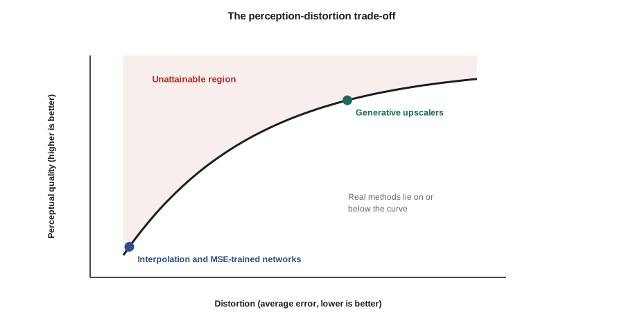
In 2018 Yochai Blau and Tomer Michaeli proved a striking result: for image restoration, there is a fundamental trade-off between distortion (how far the output is from the true image on average, as measured by MSE or similar) and perceptual quality (how much the output looks like a natural image). An algorithm that minimizes average error produces outputs that are an average of all plausible answers, which looks blurry. An algorithm that produces sharp, natural-looking outputs must commit to one plausible answer, which will on average be further from the truth. You cannot have both at their best simultaneously.
This explains why generative upscalers look sharper than classical ones yet score worse on PSNR, and why their detail can be convincingly wrong. For photographers, the practical rule is to choose the tool according to purpose. For an art print where pleasing texture matters, a perceptually optimized upscaler is appropriate. For a document where fidelity matters, choose fidelity-oriented settings, accept softness and disclose any enhancement. Many tools now offer both modes, labeled for example as "faithful" and "creative" or with a strength slider; understanding the trade-off helps you set them.
Common mistakes
MistakeAssuming AI denoising only removes noise
InsteadInspect at 100 percent for invented texture, especially at extreme ISO.
MistakeSharpening without masking
InsteadRestrict sharpening to edges so flat areas do not gain noise.
MistakeTreating upscaled detail as real
InsteadRemember single-image upscaling predicts detail; do not use it for evidence or identification.
MistakeJudging a restoration by PSNR alone
InsteadCombine PSNR, SSIM or perceptual metrics with visual inspection for the intended use.
MistakeChoosing the most pleasing result for documentary work
InsteadPrefer fidelity-oriented settings and disclose enhancement where accuracy matters.
Summary and key terms
- Classical denoisers range from Gaussian blur through bilateral filtering and non-local means to BM3D.
- Learned denoisers trained on noisy and clean pairs preserve detail far better, especially on raw data.
- Unsharp masking steepens edges but adds halos and noise; deconvolution undoes known blur but amplifies noise.
- Learned upscaling and deblurring predict detail rather than measure it.
- PSNR measures pixel error; SSIM and learned metrics match perception better; FID assesses realism of sets.
- The perception-distortion trade-off means no method can minimize error and maximize realism together.
- Choose restoration settings by purpose and disclose enhancement in contexts where fidelity matters.
- Bilateral filter
- An edge-preserving filter that weights neighbors by spatial distance and value similarity.
- Non-local means
- A denoiser that averages pixels whose surrounding patches are similar anywhere in the image.
- BM3D
- Block-matching and 3D filtering, a strong classical denoiser that filters groups of similar patches.
- Unsharp mask
- Sharpening by adding back the difference between an image and a blurred copy.
- Point spread function (PSF)
- The image of a single point, describing how a system blurs.
- Deconvolution
- Estimating an original image from a blurred one given the blur's PSF.
- Single-image super-resolution
- Predicting a higher-resolution image from one low-resolution input using learned priors.
- PSNR
- Peak signal-to-noise ratio, a logarithmic measure of mean squared error relative to the maximum value.
- SSIM
- Structural similarity index, comparing local luminance, contrast and structure.
- Perception-distortion trade-off
- The proven tension between minimizing error and maximizing natural appearance.
Practice problems
Work each problem on paper first, then reveal the answer to check.
Why does a Gaussian blur damage edges while a bilateral filter does not?
Show answer
The bilateral filter gives little weight to neighbors with very different values, such as those across an edge.
What makes non-local means different from local filters?
Show answer
It averages similar patches from anywhere in the image, not just nearby pixels.
Why do raw-domain denoisers often outperform those applied after processing?
Show answer
Noise in raw data is simpler and not yet spread by demosaicing and color correction.
Write the unsharp mask formula and say what \( \alpha \) controls.
Show answer
\( I + \alpha(I - G_\sigma * I) \); \( \alpha \) controls the amount of sharpening.
Why is deconvolution ill-posed?
Show answer
Frequencies suppressed by the blur are dominated by noise, which deconvolution amplifies.
MSE is 0.001 on a 0 to 1 scale. What is the PSNR?
Show answer
\( 10 \log_{10}(1/0.001) = 30 \) dB.
How much linear upscaling does a 20 by 30 inch print at 300 ppi need from a 6,000-pixel-wide image?
Show answer
\( 9000 / 6000 = 1.5 \) times.
Why might a sharp generative upscale score lower PSNR than a soft bicubic one?
Show answer
It commits to plausible detail that differs from the truth, increasing average error.
Name one context where AI upscaling should not be used.
Show answer
Forensic evidence, identification of faces or license plates, medical or scientific images.
What does FID measure that PSNR does not?
Show answer
How realistic a set of generated images looks compared with real images, without a reference.
Lesson quiz · 5 questions
Score 60% or more to complete this lesson.
Create a free account to save your progress, take quizzes and earn a certificate.