
ROB-410 · Lesson 10 of 12 · 28 min
Learning perception and representations
Most of the policies so far took a compact state as input: joint angles, an object position, a lane offset. Real robots see the world through cameras, and a raw image has hundreds of thousands of numbers, almost all irrelevant to the task. A grasping policy does not care about the color of the wall, but it cares a great deal about a few pixels at the edge of a mug handle. Learning directly from pixels with a small task dataset tends to overfit to exactly those irrelevant details. This lesson is about representations: compact features that capture what matters for control. It covers why representations matter, how pretrained and self-supervised vision encoders provide them, how to combine several sensors, and how world models learn to predict the consequences of actions so that a robot can plan or train in imagination.
Why representations matter
A policy can be split into an encoder \( z = f_\phi(o) \) that turns an observation into a feature vector, and a head \( a = g_\theta(z) \) that turns features into actions. Training both end to end on a few hundred demonstrations asks a small dataset to teach the network both how to see and how to act. Good representations separate those jobs: the encoder is learned from large, cheap data, perhaps millions of images or videos without any robot actions, and the head is learned from the scarce robot data. The result is better sample efficiency, better robustness to lighting and backgrounds, and better generalization to new objects.
What makes a representation good for control? It should be informative about the task-relevant state, such as object poses, contacts and the robot's own configuration; invariant to nuisance factors such as lighting, texture and camera noise; smooth, so that nearby states map to nearby features and small changes produce small action changes; and compact enough for efficient learning. ROB-340 covered deep-learning perception for detection and segmentation; here the target is features for action rather than labels for people.
| Property | Why it matters for control | How to encourage it |
|---|---|---|
| Informative | Policy needs the relevant state | Train on diverse tasks; check by probing for object pose |
| Invariant to nuisances | Robustness to lighting, textures, backgrounds | Augmentation, contrastive learning, domain randomization |
| Smooth | Stable actions and good generalization | Regularization; temporal consistency objectives |
| Compact | Fewer parameters to learn in the head | Bottleneck layers, pooling, keypoints |
| Fast to compute | Real-time control loops | Efficient backbones, smaller input sizes, caching |
Self-supervised learning
Self-supervised learning creates training signals from the data itself, with no human labels. Three families dominate vision. Contrastive methods, such as SimCLR and MoCo, take two augmented views of the same image and train the encoder so that their features are close while features of different images are far apart; the augmentations define what the representation should ignore. Masked modeling, as in masked autoencoders, hides most patches of an image and trains a network to reconstruct them, which forces it to learn the structure of scenes. Self-distillation methods, such as DINO and its successors, train a student network to match a slowly updated teacher's outputs on different crops, and produce features that capture object parts remarkably well.
The contrastive objective, often called InfoNCE, can be written for a batch of \( N \) image pairs as:
Here \( z_i \) and \( z_i^{+} \) are normalized features of two views of image \( i \), and \( \tau \) is a temperature. Minimizing the loss makes each image's two views more similar to each other than to any other image in the batch. For robots, an attractive variant uses time as the augmentation: frames close together in a video should have similar features, frames far apart should differ, and frames from different camera angles at the same moment should match. This time-contrastive learning encourages features that track the progress of a task.
# InfoNCE on toy features: matched views score far better than random features
import numpy as np
rng = np.random.default_rng(10)
def info_nce(z, zp, tau=0.1):
    z = z / np.linalg.norm(z, axis=1, keepdims=True)
    zp = zp / np.linalg.norm(zp, axis=1, keepdims=True)
    logits = z @ zp.T / tau
    logits -= logits.max(1, keepdims=True)
    logp = logits - np.log(np.exp(logits).sum(1, keepdims=True))
    return -np.mean(np.diag(logp))
N, d = 64, 16
content = rng.normal(size=(N, d))                    # what the images are "about"
view_a = content + 0.3 * rng.normal(size=(N, d))     # augmentation noise
view_b = content + 0.3 * rng.normal(size=(N, d))
random_b = rng.normal(size=(N, d))
print(f"loss with matched views : {info_nce(view_a, view_b):.3f}")
print(f"loss with random pairs  : {info_nce(view_a, random_b):.3f}")
print(f"chance level log(N) : {np.log(N):.3f}")loss with matched views : 0.106 loss with random pairs : 6.659 chance level log(N) : 4.159
Pretrained vision encoders for robots
A practical shortcut is to take an encoder pretrained on a huge image or video dataset and reuse it. General-purpose options include ImageNet-trained ResNets, self-distilled vision transformers such as DINOv2, and image-text models such as CLIP and SigLIP, whose features are aligned with language. Robot-specific encoders have also been pretrained on large collections of first-person human video, such as R3M and VC-1, with objectives chosen to emphasize manipulation-relevant features. At the time of writing, evidence on which encoder is best is mixed: results depend strongly on the task, the amount of robot data and whether the encoder is frozen or fine-tuned. Many recent policies simply use a strong general vision-language encoder, which also lets them connect to language instructions.
Two practical choices follow. A frozen encoder keeps its pretrained weights fixed and trains only the policy head; this is cheap, protects against overfitting with tiny datasets, and allows features to be cached. Fine-tuning updates the encoder too, usually with a lower learning rate; it often wins when there are thousands of demonstrations or when the robot's viewpoint differs greatly from the pretraining images. A useful check is a linear probe: freeze the encoder and fit a linear model from features to a quantity that matters, such as object position. If a linear probe cannot recover it, the policy head will struggle too.
Worked problem
Frozen or fine-tuned?
A lab has 80 demonstrations of placing parts in a fixture, recorded from a wrist camera whose close-up views look nothing like typical internet photos. A frozen encoder gives a 55 % success rate. What should the team try, and what risk should it watch?
Show solution
- The viewpoint gap suggests the frozen features may miss fine details; fine-tuning could help.
- With only 80 demonstrations, full fine-tuning risks overfitting, so use a low encoder learning rate, strong augmentation and early stopping on held-out rollouts.
- Alternatively, fine-tune only the last blocks of the encoder, or add a small adapter, keeping most weights frozen.
- Compare on real closed-loop trials with confidence intervals, not on validation loss.
Answer: Try partial fine-tuning with a low learning rate and strong augmentation, and judge by closed-loop success.
Combining sensors
Robots rarely rely on one camera. A typical manipulation setup combines a fixed overhead or third-person camera for global context, a wrist camera for fine alignment, proprioception for the arm's own joint angles and gripper width, and sometimes depth, force-torque or tactile sensors. Each modality gets its own encoder, and the features are fused, either by concatenation or, in transformer policies, by treating each feature as a token that attends to the others. Proprioception is cheap and precise and should almost always be included. Force and tactile signals are essential for contact-rich tasks such as insertion and wiping, where vision cannot see the forces involved.
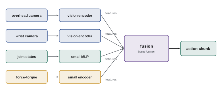
Spatial representations deserve mention. Instead of a single global feature vector, some methods extract keypoints, small sets of image coordinates that track task-relevant points such as a mug handle; others build three-dimensional point clouds or voxel grids from depth cameras and process them with networks that respect geometry. Three-dimensional representations generalize better to new camera positions and make it easier to reason about reach and collisions, at the cost of needing calibrated depth sensing.
World models
A world model learns to predict what happens next: given the current state or observation and an action, it predicts the next observation, often in a learned latent space, together with the reward. Lesson 3 described model-based RL with simple learned dynamics. Modern world models do this from images. Systems in the Dreamer family encode images into a compact latent state, learn latent dynamics with a recurrent network, and then train an actor-critic policy entirely on imagined rollouts in latent space, needing far fewer real interactions than model-free RL. Video-prediction models trained on large video collections are also being explored, at the time of writing, as general simulators that can evaluate or train policies from pixels.
# A tiny learned latent world model: fit linear dynamics, then plan by random shooting
import numpy as np
rng = np.random.default_rng(12)
A_true = np.array([[1.0, 0.1], [0.0, 0.95]]); B_true = np.array([[0.0], [0.1]])
Z, U, Zn = [], [], []
z = np.zeros(2)
for t in range(500):                                  # random exploration data
    u = rng.uniform(-1, 1, 1)
    zn = A_true @ z + B_true @ u + rng.normal(0, 0.01, 2)
    Z.append(z); U.append(u); Zn.append(zn)
    z = zn if np.abs(zn).max() < 3 else np.zeros(2)
X = np.hstack([np.array(Z), np.array(U)])
M, *_ = np.linalg.lstsq(X, np.array(Zn), rcond=None)
A_hat, B_hat = M[:2].T, M[2:].T
print("learned A:\n", np.round(A_hat, 3), "\nlearned B:", np.round(B_hat.ravel(), 3))
goal, z = np.array([1.0, 0.0]), np.zeros(2)
for step in range(40):                                # model predictive control in the learned model
    seqs = rng.uniform(-1, 1, size=(256, 10))
    costs = np.zeros(256)
    for k in range(256):
        zz = z.copy()
        for u in seqs[k]:
            zz = A_hat @ zz + B_hat.ravel() * u
            costs[k] += np.sum((zz - goal) ** 2)
    u0 = seqs[np.argmin(costs), 0]
    z = A_true @ z + B_true.ravel() * u0              # act in the real system
print("final state after 40 steps:", np.round(z, 3))learned A: [[0.999 0.101] [0.001 0.953]] learned B: [0.001 0.099] final state after 40 steps: [0.915 0.066]
Worked problem
Model error over an imagined horizon
A learned world model's one-step prediction error is about 2 % of the state scale, and errors grow roughly additively. A planner imagines 15 steps ahead. Roughly how large is the error at the end of the horizon, and what does this suggest?
Show solution
- Additive growth: \( 15 \times 2\% = 30\% \) of the state scale by step 15.
- Errors can grow faster than additively if they move the model into poorly covered states.
- Plan over shorter horizons, replan every step, use ensembles to detect uncertainty, and keep collecting real data where the model is wrong.
Answer: Roughly 30 % of the state scale, so long imagined horizons are unreliable; short horizons with frequent replanning are safer.
World models face the same issue as lesson 3's simple models: errors compound over imagined horizons, and a policy optimized in an imperfect model will exploit the model's errors, just as RL exploits simulator quirks. Ensembles of models, short horizons, uncertainty penalties and periodic real-world data collection keep this in check.
Common mistakes
MistakeTraining a vision policy from scratch on a few hundred demonstrations.
InsteadStart from a pretrained encoder and add augmentation; train from scratch only with abundant data.
MistakeFine-tuning a large encoder at the same learning rate as the head.
InsteadUse a lower encoder learning rate or freeze most layers when data is scarce.
MistakeLeaving out proprioception.
InsteadJoint states are cheap, precise and almost always improve manipulation policies.
MistakeChoosing augmentations without thinking about the task.
InsteadAugmentations define invariances; random crops that cut off the gripper or color jitter on a color-sorting task remove information the policy needs.
MistakeTrusting long imagined rollouts in a learned world model.
InsteadUse short horizons, replanning, ensembles and continued real data collection.
Summary and key terms
- Representations compress observations into features that capture what matters for control.
- Good features are informative, invariant to nuisances, smooth, compact and fast.
- Self-supervised learning uses contrastive, masked and self-distillation objectives without labels.
- Pretrained encoders, frozen or fine-tuned, improve sample efficiency and robustness.
- Linear probes check whether features contain task-relevant information.
- Multi-sensor policies fuse cameras, proprioception and force with separate encoders.
- World models predict latent dynamics for planning or imagined training, but their errors compound.
- Representation
- A learned feature vector summarizing an observation.
- Encoder
- A network mapping raw observations to features.
- Self-supervised learning
- Learning from training signals derived from the data itself.
- Contrastive learning
- Pulling features of related views together and pushing unrelated ones apart.
- InfoNCE
- A contrastive loss that scores the matched pair against others in a batch.
- Masked autoencoder
- A model trained to reconstruct hidden patches of an input.
- Linear probe
- A linear model fitted on frozen features to test what they encode.
- Proprioception
- The robot's sensing of its own joint positions and velocities.
- Sensor fusion
- Combining features from several sensing modalities.
- World model
- A learned model that predicts future observations or latent states given actions.
Practice problems
Work each problem on paper first, then reveal the answer to check.
Why separate an encoder from a policy head?
Show answer
The encoder can learn from large cheap data and the head from scarce robot data.
What defines the invariances in contrastive learning?
Show answer
The augmentations used to create the two views.
What does a masked autoencoder reconstruct?
Show answer
Hidden patches of the input image.
What is chance-level InfoNCE loss for a batch of 128?
Show answer
\( \log 128 \approx 4.85 \).
When is fine-tuning an encoder most likely to help?
Show answer
With plenty of robot data or a large viewpoint gap from pretraining images.
What does a linear probe test?
Show answer
Whether frozen features contain a quantity recoverable by a linear model.
Why include a wrist camera as well as an overhead one?
Show answer
It gives close-up views for fine alignment.
Which sensors matter most for insertion tasks?
Show answer
Force-torque or tactile sensors.
What does Dreamer train its policy on?
Show answer
Imagined rollouts in a learned latent world model.
A model has 3 % one-step error. Additive error after 10 steps?
Show answer
About 30 %.
Lesson quiz · 5 questions
Score 60% or more to complete this lesson.
Create a free account to save your progress, take quizzes and earn a certificate.