
ROB-410 · Lesson 4 of 12 · 30 min
Reinforcement learning I: value-based methods
Dynamic programming needs a model of the world. Most robots do not have an accurate one, especially when contact, deformable objects or unknown terrain are involved. Model-free reinforcement learning removes that requirement: the agent estimates values directly from its own experience, one transition at a time. This lesson covers the value-based branch of model-free RL, from temporal-difference learning and tabular Q-learning to the deep Q-network ideas that made learning from pixels practical, and the exploration problem that every RL agent must solve. Lesson 5 covers the other branch, which learns policies directly.
Learning from experience instead of a model
Suppose the robot does not know \( P(s' \mid s, a) \) but can try actions and see what happens. One way to estimate \( V^\pi(s) \) is Monte Carlo evaluation: run complete episodes under \( \pi \), record the return that followed each visit to \( s \), and average those returns. Monte Carlo estimates are unbiased, but they have high variance, because a single return depends on every random event for the rest of the episode, and they cannot be computed until the episode ends.
Temporal-difference learning, or TD learning, updates estimates after every step instead. It uses the Bellman recursion: the value of the current state should equal the reward just received plus the discounted value of the next state. The gap between that one-step target and the current estimate is the TD error, \( \delta \), and the estimate is nudged toward the target by a step size \( \alpha \):
Because TD uses its own current estimate of \( V(s_{t+1}) \) inside the target, it is said to bootstrap. Bootstrapping introduces bias, since the estimate may be wrong, but it greatly reduces variance and lets learning happen online, during an episode. Methods that blend the two, such as \( n \)-step returns and TD(\( \lambda \)), sit between Monte Carlo and one-step TD and are widely used in practice.
Worked problem
A single TD update
A robot's current estimate is \( V(s) = 4.0 \) and \( V(s') = 6.0 \). It takes an action, receives reward −0.5 and lands in \( s' \). With \( \gamma = 0.9 \) and \( \alpha = 0.1 \), compute the TD error and the new \( V(s) \).
Show solution
- Target: \( -0.5 + 0.9 \times 6.0 = 4.9 \).
- TD error: \( \delta = 4.9 - 4.0 = 0.9 \).
- Update: \( V(s) \gets 4.0 + 0.1 \times 0.9 = 4.09 \).
Answer: \( \delta = 0.9 \) and the new estimate is 4.09. The positive TD error means things went better than expected, so the estimate moves up.
Q-learning
Estimating \( V \) is not enough to choose actions without a model, because choosing the best action from \( V \) requires knowing where each action leads. Estimating \( Q(s, a) \) solves that problem: the best action is simply the one with the largest \( Q \). Q-learning applies a TD update to action values, using the Bellman optimality equation for the target:
Q-learning is off-policy: its target uses the best action in the next state, regardless of which action the agent actually takes next. That means the agent can behave in one way, for example exploring randomly, while learning the values of the optimal policy. Under conditions that include visiting every state-action pair infinitely often and reducing the step size appropriately, tabular Q-learning converges to \( Q^* \). Its on-policy cousin, SARSA, uses the action actually taken next, \( Q(s_{t+1}, a_{t+1}) \), and therefore learns the value of the behavior policy, including its exploration. SARSA tends to learn more cautious policies near hazards, because it accounts for the occasional random step.
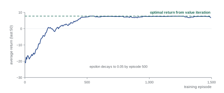
# Tabular Q-learning on a 4x4 gridworld (goal top-right, trap below it)
import numpy as np
rng = np.random.default_rng(0)
n, gamma, alpha = 4, 0.95, 0.2
goal, trap = (0, 3), (1, 3)
moves = [(-1, 0), (1, 0), (0, -1), (0, 1)]          # up, down, left, right
def step(s, a):
    if rng.random() < 0.1:                            # 10 % chance the move fails
        s2 = s
    else:
        r, c = s[0] + moves[a][0], s[1] + moves[a][1]
        s2 = (r, c) if 0 <= r < n and 0 <= c < n else s
    if s2 == goal: return s2, 10.0, True
    if s2 == trap: return s2, -10.0, True
    return s2, -0.4, False
Q = np.zeros((n, n, 4))
returns = []
for ep in range(1500):
    eps = max(0.05, 1.0 - ep / 500)                   # decaying epsilon-greedy
    s, G, done, t = (3, 0), 0.0, False, 0
    while not done and t < 100:
        a = rng.integers(4) if rng.random() < eps else int(np.argmax(Q[s]))
        s2, r, done = step(s, a)
        target = r if done else r + gamma * Q[s2].max()
        Q[s][a] += alpha * (target - Q[s][a])
        s, G, t = s2, G + r, t + 1
    returns.append(G)
print("avg return, first 100 episodes:", round(np.mean(returns[:100]), 2))
print("avg return, last 100 episodes: ", round(np.mean(returns[-100:]), 2))
print("learned V = max_a Q:")
print(np.round(Q.max(axis=2), 2))avg return, first 100 episodes: -14.57 avg return, last 100 episodes: 7.11 learned V = max_a Q: [[8.07 8.98 9.98 0. ] [7.12 7.88 9.05 0. ] [6.39 7.21 8.05 7.12] [5.61 6.26 6.88 6.33]]
Compare the learned values with the value-iteration result from lesson 3 for the same gridworld. They should be close in the states the agent visited often and less accurate in rarely visited corners, which is typical: model-free methods learn well only where they have data.
Exploration and exploitation
An agent that always takes the action it currently believes is best will never discover that another action is better. An agent that always explores will never use what it has learned. Balancing the two is the exploration-exploitation dilemma. The simplest strategy is \( \epsilon \)-greedy: take a random action with probability \( \epsilon \) and the greedy action otherwise, usually decaying \( \epsilon \) from near 1 to a small value as learning proceeds. Other strategies include Boltzmann (softmax) exploration over Q-values, optimism in the face of uncertainty, where untried actions are assumed to be good until proven otherwise, and intrinsic-motivation bonuses that reward visiting novel states.
On real robots, random exploration is often unacceptable. A random joint command can drive an arm into a table or a person. Robot RL therefore restricts exploration in several ways: limiting actions to small changes around a safe controller, adding noise in a smooth, low-frequency way rather than as independent jumps at each step, enforcing hard safety limits outside the learner, exploring in simulation first, or starting from a policy learned by imitation so that exploration is concentrated near sensible behavior. Lesson 6 returns to safe exploration.
Worked problem
How much exploration remains?
An agent uses \( \epsilon \)-greedy with \( \epsilon = 0.1 \) and four actions. What fraction of steps take a non-greedy action? In a 200-step episode, how many such steps should you expect?
Show solution
- A random action is taken with probability 0.1, but one time in four the random action happens to be the greedy one.
- Probability of a non-greedy action: \( 0.1 \times 3/4 = 0.075 \).
- Expected non-greedy steps in 200: \( 200 \times 0.075 = 15 \).
Answer: About 7.5 % of steps, or 15 per 200-step episode. On a real robot, each of those 15 random actions must be safe.
Function approximation and deep Q-networks
Tables cannot represent values over continuous or high-dimensional states such as camera images. Instead, we approximate \( Q(s, a) \) with a parameterized function \( Q_\theta(s, a) \), often a neural network, and update its parameters \( \theta \) to reduce the TD error by gradient descent. With a network that takes an image and outputs one Q-value per discrete action, a single forward pass gives the values of all actions.
Naively combining Q-learning with neural networks is unstable. Consecutive samples are highly correlated, and the target \( r + \gamma \max_{a'} Q_\theta(s', a') \) changes every time \( \theta \) changes, so the network chases a moving target. The deep Q-network, or DQN, introduced two fixes that are now standard. Experience replay stores transitions in a large buffer and trains on random mini-batches drawn from it, breaking correlations and reusing each transition many times. A target network, a slowly updated copy of the Q-network, computes the targets, so they stay steady for many updates. A third common fix, double Q-learning, reduces the systematic overestimation that comes from taking a maximum over noisy estimates, by using one network to choose the best next action and another to evaluate it.
In this double-DQN loss, \( \mathcal{D} \) is the replay buffer, \( \theta \) are the online network parameters and \( \bar{\theta} \) are the target network parameters. Large-scale robot grasping systems in the late 2010s used variants of this idea, with continuous actions handled by sampling candidate actions and choosing the one with the highest predicted Q-value, trained on hundreds of thousands of real grasp attempts collected by fleets of arms.
# PyTorch-style DQN update (listing only, not run here)
import torch, torch.nn.functional as F
def dqn_update(q_net, target_net, optimizer, batch, gamma=0.99):
    s, a, r, s2, done = batch                           # tensors from the replay buffer
    q = q_net(s).gather(1, a.unsqueeze(1)).squeeze(1)   # Q(s, a) for the actions taken
    with torch.no_grad():
        a2 = q_net(s2).argmax(dim=1, keepdim=True)      # double DQN: online net chooses
        q2 = target_net(s2).gather(1, a2).squeeze(1)    # target net evaluates
        target = r + gamma * (1.0 - done) * q2
    loss = F.smooth_l1_loss(q, target)
    optimizer.zero_grad(); loss.backward(); optimizer.step()
    return loss.item()
# Every N steps: target_net.load_state_dict(q_net.state_dict())| Problem | Symptom | Standard fix |
|---|---|---|
| Correlated consecutive samples | Unstable or diverging training | Experience replay with random mini-batches |
| Moving targets | Oscillating Q-values | Slowly updated target network |
| Maximization bias | Systematically overestimated values | Double Q-learning |
| Rare rewards | No learning signal for long periods | Shaped rewards, demonstrations, hindsight relabeling |
| Continuous actions | Max over actions is intractable | Sampled actions, or actor-critic methods (lesson 5) |
Sparse rewards and hindsight
Robot tasks often have sparse rewards: the robot is told only whether it succeeded. Early in training it almost never succeeds, so nearly every reward is zero and nothing is learned. Hindsight experience replay offers a clever partial fix for goal-conditioned tasks, such as reaching a commanded position. When an episode fails to reach the intended goal, the transitions are stored a second time as if the goal had been wherever the robot actually ended up. Those relabeled transitions are successes, so the agent learns how to reach many goals, which in turn helps it reach the one it was asked for. Demonstrations, curricula that start with easy goals, and shaped rewards are other standard responses, and lessons 6 to 9 develop them further.
Worked problem
How rare is success under random exploration?
A gripper must close within 1 cm of an object's center along one axis. Random exploration places the gripper uniformly over a 40 cm span. Ignoring the other axes, what is the chance of success per attempt? With three independent axes of the same size, what is it?
Show solution
- One axis: the success window is 2 cm wide (±1 cm) out of 40 cm, so \( 2/40 = 0.05 \).
- Three axes: \( 0.05^3 = 1.25 \times 10^{-4} \), about one success in 8,000 attempts.
- Adding orientation requirements would make it rarer still.
Answer: About 5 % on one axis but only about 1 in 8,000 with three axes, which is why sparse-reward manipulation needs hindsight, demonstrations or shaping.
Strengths and limits of value-based methods
Value-based methods are sample-efficient compared with many policy-gradient methods, because they can reuse old data from a replay buffer. They work naturally with discrete actions, such as choosing which object to pick, which grasp from a ranked list to try, or which high-level skill to run next. Their weaknesses for low-level robot control are that taking a maximum over continuous actions is awkward, that training can be unstable, and that small errors in value estimates can produce brittle policies. For continuous control, most current robot RL uses actor-critic methods, which combine a learned value function with an explicitly parameterized policy. Those are the subject of lesson 5.
Common mistakes
MistakeNever decaying \( \epsilon \), or decaying it to zero too fast.
InsteadDecay gradually and keep a small floor so the agent continues to explore states it has rarely seen.
MistakeTraining a Q-network on consecutive samples.
InsteadUse experience replay so mini-batches are diverse and transitions are reused.
MistakeComputing targets with the same network being trained.
InsteadUse a target network that is updated slowly or periodically.
MistakeLetting a real robot explore with independent random jumps.
InsteadConstrain exploration with smooth noise, small action limits, external safety checks and simulation first.
MistakeTrusting value estimates in rarely visited states.
InsteadModel-free values are reliable only where there is data; collect more there or restrict the policy to familiar states.
Summary and key terms
- Model-free RL estimates values from experience without a transition model.
- Monte Carlo averages complete returns; TD learning bootstraps from the next state's estimate after every step.
- Q-learning learns optimal action values off-policy; SARSA learns the values of the behavior policy.
- Exploration strategies balance trying new actions with exploiting known good ones; on robots, exploration must be constrained for safety.
- Deep Q-networks use function approximation with experience replay and target networks; double Q-learning reduces overestimation.
- Sparse rewards make learning slow; hindsight relabeling, demonstrations and shaping help.
- Value-based methods suit discrete decisions; continuous control usually uses actor-critic methods.
- Model-free RL
- Reinforcement learning that learns values or policies directly from experience, without a dynamics model.
- Temporal-difference learning
- Updating value estimates toward a target built from the next reward and the next state's estimate.
- TD error
- The difference between the one-step target and the current value estimate.
- Bootstrapping
- Using current value estimates inside the targets used to update them.
- Q-learning
- An off-policy TD method that learns optimal action values using a max over next actions.
- SARSA
- An on-policy TD method whose target uses the action actually taken next.
- Epsilon-greedy
- Choosing a random action with probability epsilon and the greedy action otherwise.
- Experience replay
- Storing transitions in a buffer and training on random mini-batches from it.
- Target network
- A slowly updated copy of the value network used to compute stable targets.
- Hindsight experience replay
- Relabeling failed episodes with the goals they actually achieved so they count as successes.
Practice problems
Work each problem on paper first, then reveal the answer to check.
\( V(s) = 2 \), \( V(s') = 3 \), reward 1, \( \gamma = 1 \), \( \alpha = 0.5 \). New \( V(s) \)?
Show answer
Target 4, error 2, new value \( 2 + 0.5 \times 2 = 3 \).
Why is Q-learning called off-policy?
Show answer
Its target uses the greedy next action, not the action the behavior policy actually takes.
What does experience replay fix?
Show answer
Correlation between consecutive samples, and it allows data reuse.
What does a target network fix?
Show answer
The instability of chasing targets that change with every update.
Why do max operators overestimate values?
Show answer
Taking the maximum of noisy estimates picks up positive noise.
With \( \epsilon = 0.2 \) and five actions, what fraction of steps are non-greedy?
Show answer
\( 0.2 \times 4/5 = 0.16 \).
Name two safe-exploration measures for real robots.
Show answer
Small action limits, smooth noise, external safety checks, simulation first, or starting from demonstrations.
What does hindsight experience replay do with a failed reach?
Show answer
Stores it again with the achieved position as the goal, turning it into a success.
Why do value-based methods struggle with continuous actions?
Show answer
The max over a continuous action space is hard to compute.
Which is more conservative near a cliff, SARSA or Q-learning?
Show answer
SARSA, because it accounts for exploratory steps.
Lesson quiz · 5 questions
Score 60% or more to complete this lesson.
Create a free account to save your progress, take quizzes and earn a certificate.