
ROB-410 · Lesson 8 of 12 · 29 min
Imitation learning I: behavior cloning and DAgger
Reinforcement learning discovers behavior from rewards, which is powerful but slow and dependent on a well-designed reward. Often there is a faster route: a person already knows how to do the task and can show the robot. Imitation learning trains a policy from demonstrations. For manipulation in particular it has become the dominant approach at the time of writing (October 2026), because writing a reward for folding a shirt or loading a dishwasher is hard, while demonstrating it is easy. This lesson covers the simplest form, behavior cloning, explains why it fails in a characteristic way, and presents DAgger, an algorithm that fixes the failure by collecting corrections where the policy actually goes.
Behavior cloning as supervised learning
Behavior cloning treats imitation as supervised learning. A demonstrator, usually a person teleoperating the robot, performs the task many times while the system records observation-action pairs \( (o_t, a_t) \). The dataset \( \mathcal{D} = \{(o_i, a_i)\} \) is then used to train a policy \( \pi_\theta(a \mid o) \) by minimizing a loss between the policy's output and the demonstrated action.
For continuous actions the loss \( \ell \) is often mean squared error, which corresponds to a Gaussian policy with fixed variance; for discrete actions it is cross-entropy. Everything you know from supervised learning applies: train and validation splits, regularization, data augmentation and model capacity. The appeal is obvious. There is no reward, no exploration and no simulator; given a few hundred demonstrations, a standard network can learn surprisingly capable behavior in hours.
# Cloning an expert by linear regression on synthetic demonstrations
import numpy as np
rng = np.random.default_rng(8)
# Expert: a proportional controller that drives a 2-D point to the origin
K_expert = np.array([[-1.2, 0.0], [0.0, -0.8]])
def expert(s):
    return K_expert @ s
S = rng.uniform(-1, 1, size=(200, 2))                       # demonstrated states
A = S @ K_expert.T + rng.normal(0, 0.05, size=(200, 2))    # demonstrated actions (noisy)
X = np.hstack([S, np.ones((200, 1))])                       # add a bias column
W, *_ = np.linalg.lstsq(X, A, rcond=None)                   # least-squares fit
print("learned gain matrix:\n", np.round(W[:2].T, 3))
print("learned bias:", np.round(W[2], 3))
test = np.array([0.5, -0.4])
print("expert action :", np.round(expert(test), 3))
print("cloned action :", np.round(np.append(test, 1) @ W, 3))learned gain matrix: [[-1.194e+00 1.000e-03] [ 1.000e-02 -8.060e-01]] learned bias: [-0. 0.002] expert action : [-0.6 0.32] cloned action : [-0.598 0.33 ]
When the expert is linear and the states are well covered, as here, behavior cloning recovers it almost exactly. Real experts are neither linear nor perfectly consistent, and real datasets cover only a thin band of the state space. That is where the trouble starts.
Distribution shift and compounding errors
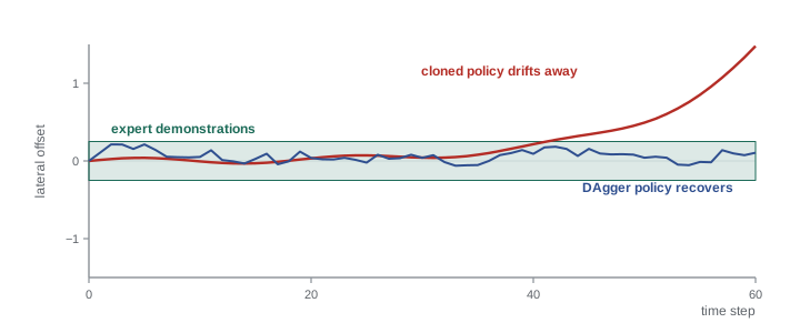
Supervised learning assumes that the test inputs come from the same distribution as the training inputs. Behavior cloning breaks this assumption. The training states come from the expert's trajectories; the test states come from the learned policy's own trajectories. Any small error the policy makes moves it slightly away from where the expert would have been, into a state that appears rarely or never in the data. There its prediction is worse, so the next error is larger, which moves it further away. Errors compound.
The classic analysis by Ross and Bagnell makes this precise. If the cloned policy makes a mistake with probability \( \epsilon \) on states drawn from the expert's distribution, then over a task of horizon \( T \) the expected number of mistakes can grow as \( O(\epsilon T^2) \), rather than the \( O(\epsilon T) \) one would expect if every state were drawn from the training distribution. Doubling the task length can quadruple the errors.
Here \( J \) is the expected total cost. The quadratic term is the compounding error. It explains a pattern every practitioner sees: a cloned policy that follows the demonstrations well for the first few seconds, drifts slightly, then fails catastrophically because it has never seen how to recover from the drifted state.
Worked problem
How compounding error scales
A cloned policy errs with probability 0.01 per step on expert-like states. Compare rough expected mistake counts for horizons of 50 and 200 steps under linear and quadratic growth.
Show solution
- Linear growth: \( \epsilon T = 0.5 \) at 50 steps and 2 at 200 steps.
- Quadratic growth: \( \epsilon T^2 = 25 \) at 50 steps and 400 at 200 steps (as a bound on accumulated cost, not literal counts).
- Quadrupling the horizon multiplies the linear term by 4 but the quadratic term by 16.
Answer: Long-horizon tasks are where behavior cloning is most fragile; the gap between linear and quadratic growth widens rapidly with \( T \).
DAgger: dataset aggregation
DAgger, introduced by Ross, Gordon and Bagnell in 2011, attacks the root cause. If the policy will visit states the expert never visited, then ask the expert what to do in those states. The algorithm alternates between running the current policy and labeling the states it visits with expert actions.
| Step | What happens |
|---|---|
| 1 | Collect expert demonstrations into dataset \( \mathcal{D} \) and train an initial policy \( \pi_1 \) by behavior cloning. |
| 2 | Run \( \pi_i \) (optionally mixed with the expert) and record the states it visits. |
| 3 | Ask the expert to label each visited state with the action it would have taken. |
| 4 | Add these labeled pairs to \( \mathcal{D} \), the aggregated dataset. |
| 5 | Retrain on all of \( \mathcal{D} \) to obtain \( \pi_{i+1} \), and repeat from step 2. |
Because the dataset grows to include states from the learner's own distribution, the policy learns how to recover from its own mistakes. Theory shows the cost grows only linearly in the horizon. In practice a handful of iterations often transforms a fragile cloned policy into a robust one.
# DAgger illustration: a 1-D lane-keeping task with a lookup-table learner
import numpy as np
rng = np.random.default_rng(11)
def expert(x):
    return -np.tanh(2.0 * x)              # steer back toward the middle of the lane
edges = np.linspace(-3, 3, 121)          # a lookup-table policy over 120 bins
def fit(X, Y):
    idx = np.digitize(X, edges)
    table = {i: Y[idx == i].mean() for i in set(idx)}
    return lambda x: table.get(int(np.digitize(x, edges)), 0.0)   # unseen bin: no steering
def rollout(policy, T=80, x0=0.0, noise=0.06):
    x, xs = x0, []
    for _ in range(T):
        xs.append(x)
        x = x + 0.5 * policy(x) + rng.normal(0, noise)
    return np.array(xs)
X = rng.normal(0, 0.04, 300)             # expert demonstrations stay very close to the middle
Y = expert(X)
pi = fit(X, Y)
for it in range(5):
    errs = [np.mean(np.abs(rollout(pi))) for _ in range(200)]
    print(f"iteration {it}: dataset {len(X):4d}, mean |offset| {np.mean(errs):.3f}")
    xs = np.concatenate([rollout(pi) for _ in range(5)])   # states the learner visits
    X, Y = np.append(X, xs), np.append(Y, expert(xs))      # expert labels them
    pi = fit(X, Y)
print(f"expert itself : mean |offset| {np.mean([np.mean(np.abs(rollout(expert))) for _ in range(200)]):.3f}")iteration 0: dataset 300, mean |offset| 0.173 iteration 1: dataset 700, mean |offset| 0.048 iteration 2: dataset 1100, mean |offset| 0.049 iteration 3: dataset 1500, mean |offset| 0.049 iteration 4: dataset 1900, mean |offset| 0.049 expert itself : mean |offset| 0.047
Worked problem
Reading the DAgger output
In the output above, why is the first iteration's error the largest, and why does it fall afterwards even though the expert itself never changes?
Show solution
- Iteration 0 uses only expert data concentrated very close to the middle of the lane; the lookup table has no entries farther out and outputs no steering there.
- When noise pushes the car outward, the cloned policy does nothing and drifts further, so its mean offset is several times the expert's.
- DAgger adds those outer states with correct expert labels, so after one iteration the learner matches the expert's mean offset of about 0.05.
Answer: The error falls because the training distribution expands to match the states the policy actually visits.
DAgger in practice
Classic DAgger requires the expert to label states after the fact, which is awkward for a person: it is hard to say what steering angle you would have used when watching a recording. Practical variants address this. In human-gated DAgger, often called HG-DAgger, the robot runs its policy while a person watches and takes over only when it is about to fail; the takeover segments become new training data. This is natural for teleoperation systems and also improves safety. Interactive correction interfaces let operators nudge the robot through a spacemouse or a leader arm. In simulation, a scripted or privileged expert, like the teacher in lesson 7's teacher-student training, can label any state automatically, which is why DAgger is the standard way to distil privileged teachers into deployable students.
Worked problem
Planning a correction campaign
A cloned bin-picking policy succeeds on 62 of 100 trials. An operator supervises with HG-DAgger and intervenes on average 1.5 times per failed trial, each intervention producing about 8 s of correction data. How much correction data does one round of 100 trials yield?
Show solution
- Failures: 38 trials.
- Interventions: \( 38 \times 1.5 = 57 \).
- Data: \( 57 \times 8 = 456 \) s, about 7.6 minutes, concentrated exactly where the policy fails.
Answer: About 7.6 minutes of targeted correction data per round, typically far more valuable per second than additional ordinary demonstrations.
Other remedies for distribution shift
DAgger is not the only defense. Noise injection during demonstration, known as DART, perturbs the expert's actions while recording so that the data naturally includes recovery from small deviations. Data augmentation for images, such as random crops and color jitter, widens visual coverage. Predicting short sequences of future actions rather than one action at a time, called action chunking, reduces the number of decisions per task and so the opportunities for errors to compound; lesson 9 meets it in ACT and Diffusion Policy. Finally, high-quality, consistent demonstrations matter enormously: a policy cannot be better than its data, and mixed strategies from different operators can confuse a regression model, a problem lesson 9 addresses with generative policies.
| Remedy | How it helps | Cost |
|---|---|---|
| DAgger | Labels learner-visited states | Expert must label or supervise repeatedly |
| HG-DAgger | Operator intervenes only near failure | Requires a takeover interface and supervision time |
| Noise injection (DART) | Demonstrations include recoveries | Slightly degraded demonstrations |
| Data augmentation | Wider visual coverage | Little; careful choice of augmentations |
| Action chunking | Fewer decisions, smoother actions | Less reactive within a chunk |
| More consistent demonstrations | Cleaner, unimodal targets | Operator training and protocols |
# PyTorch BC training step with image observations (listing only)
import torch, torch.nn as nn
policy = nn.Sequential(encoder, nn.Linear(512, 256), nn.ReLU(), nn.Linear(256, action_dim))
opt = torch.optim.AdamW(policy.parameters(), lr=1e-4, weight_decay=1e-4)
for images, proprio, actions in loader:               # LeRobot or custom dataset
    images = augment(images)                          # random crop, brightness jitter
    pred = policy(torch.cat([images_feat(images), proprio], dim=-1))
    loss = nn.functional.mse_loss(pred, actions)
    opt.zero_grad(); loss.backward(); opt.step()
Common mistakes
MistakeTreating low validation loss as proof the policy works.
InsteadValidation states come from the expert; only closed-loop rollouts reveal compounding errors.
MistakeCollecting only perfect demonstrations.
InsteadInclude recoveries, through noise injection or corrections, so the policy learns to return to the task.
MistakeMixing operators with different strategies in one regression model.
InsteadStandardize demonstration protocols or use a generative policy that can represent several modes.
MistakeAsking people to label recorded states offline.
InsteadUse human-gated interventions, where operators take over live when the robot is about to fail.
MistakeAssuming more of the same demonstrations will fix drift.
InsteadTarget data at the states the policy actually visits, as DAgger does.
Summary and key terms
- Imitation learning trains policies from demonstrations, avoiding reward design and exploration.
- Behavior cloning is supervised regression or classification from observations to actions.
- Distribution shift occurs because the policy visits states the expert never did.
- Compounding errors can grow quadratically with horizon for behavior cloning.
- DAgger aggregates expert labels on learner-visited states, reducing the growth to linear.
- Human-gated interventions make DAgger practical with people as experts.
- Noise injection, augmentation, action chunking and consistent data also reduce drift.
- Imitation learning
- Learning a policy from demonstrations of the desired behavior.
- Behavior cloning
- Supervised learning of a mapping from observations to demonstrated actions.
- Demonstration
- A recorded sequence of observations and expert actions.
- Distribution shift
- A mismatch between training-time and deployment-time input distributions.
- Compounding error
- Growth of errors as small deviations lead to unfamiliar states.
- DAgger
- Dataset Aggregation: iteratively labeling learner-visited states with expert actions.
- HG-DAgger
- A variant in which a human intervenes only when the robot is about to fail.
- DART
- Injecting noise into expert actions during demonstration so data includes recoveries.
- Action chunking
- Predicting a short sequence of future actions at each decision.
- Teleoperation
- Controlling a robot remotely, commonly used to collect demonstrations.
Practice problems
Work each problem on paper first, then reveal the answer to check.
What loss is typical for continuous-action behavior cloning?
Show answer
Mean squared error.
Why does supervised learning's main assumption fail for cloning?
Show answer
Test states come from the policy's own distribution, not the expert's.
How does compounding error scale with horizon for behavior cloning?
Show answer
Up to quadratically, \( O(\epsilon T^2) \).
What does DAgger add to the dataset each iteration?
Show answer
States visited by the learner, labeled with expert actions.
Why is HG-DAgger easier for people than classic DAgger?
Show answer
They intervene live instead of labeling recorded states.
Name a remedy for drift that does not require a second round of data.
Show answer
Noise injection, augmentation or action chunking.
A policy succeeds 70 of 100 times; failures average 2 interventions of 5 s. How much correction data?
Show answer
\( 30 \times 2 \times 5 = 300 \) s.
Why is low validation loss misleading?
Show answer
It is measured on expert states, not closed-loop rollouts.
What kind of expert labels states automatically in simulation?
Show answer
A scripted or privileged teacher policy.
Why can mixing operators hurt a regression policy?
Show answer
Averaging different strategies gives an action no operator would take.
Lesson quiz · 5 questions
Score 60% or more to complete this lesson.
Create a free account to save your progress, take quizzes and earn a certificate.