
ROB-410 · Lesson 3 of 12 · 30 min
Dynamic programming and model-based control
When the transition model and reward function of an MDP are known, the Bellman equations can be solved by computation rather than by trial and error. The family of methods that does this is called dynamic programming. It matters to robot learning for three reasons. It gives the cleanest view of what reinforcement learning algorithms are trying to approximate. It connects reinforcement learning to the optimal control you met in ROB-300, where the linear quadratic regulator turns out to be dynamic programming for a special class of problems. And it is the core of model-based reinforcement learning, in which a robot learns a model of its dynamics from data and then plans with it.
Value iteration
Value iteration starts with an arbitrary value estimate, often all zeros, and repeatedly applies the Bellman optimality equation as an update to every state:
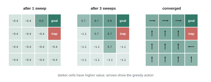
Each sweep is called a Bellman backup. Because the update is a contraction when \( \gamma < 1 \), the error shrinks by at least a factor of \( \gamma \) on every sweep, so the estimates converge to \( V^* \) from any starting point. After convergence, the optimal policy is read off by choosing the action that achieves the maximum in each state. In practice, iteration stops when the largest change in any state's value falls below a small tolerance.
A useful way to see value iteration is as information spreading outwards from rewarding states. After one sweep, only states adjacent to the goal know that the goal is nearby. After \( k \) sweeps, states up to \( k \) steps away have useful values. This is why sparse, distant rewards make learning slow: information about success has to propagate through many states.
Worked problem
One Bellman backup by hand
In state \( s \), action \( a_1 \) gives reward −1 and reaches \( s_A \) with probability 0.8 or \( s_B \) with probability 0.2. Action \( a_2 \) gives reward −1 and reaches \( s_B \) with certainty. Current estimates are \( V(s_A) = 10 \) and \( V(s_B) = 4 \), and \( \gamma = 0.9 \). What is the updated \( V(s) \) and which action is greedy?
Show solution
- For \( a_1 \): \( -1 + 0.9(0.8 \times 10 + 0.2 \times 4) = -1 + 0.9 \times 8.8 = 6.92 \).
- For \( a_2 \): \( -1 + 0.9 \times 4 = 2.6 \).
- The maximum is 6.92, from \( a_1 \).
Answer: \( V(s) \gets 6.92 \), and the greedy action is \( a_1 \).
# Value iteration on a 4x4 gridworld with slippery moves
import numpy as np
n, gamma, slip = 4, 0.95, 0.1
goal, trap = (0, 3), (1, 3)
moves = {'U': (-1, 0), 'D': (1, 0), 'L': (0, -1), 'R': (0, 1)}
def step(s, d):
    r, c = s[0] + d[0], s[1] + d[1]
    return (r, c) if 0 <= r < n and 0 <= c < n else s
def reward(s2):
    return 10.0 if s2 == goal else (-10.0 if s2 == trap else -0.4)
V = np.zeros((n, n))
for sweep in range(1, 200):
    Vn = V.copy()
    for r in range(n):
        for c in range(n):
            s = (r, c)
            if s in (goal, trap):
                continue
            best = -1e9
            for a, d in moves.items():
                # intended move with prob 1-slip, otherwise stay put
                q = 0.0
                for d2, p in ((d, 1 - slip), ((0, 0), slip)):
                    s2 = step(s, d2)
                    q += p * (reward(s2) + gamma * (0 if s2 in (goal, trap) else V[s2]))
                best = max(best, q)
            Vn[s] = best
    delta = np.abs(Vn - V).max(); V = Vn
    if delta < 1e-6:
        break
print("sweeps to converge:", sweep)
print(np.round(V, 2))sweeps to converge: 16 [[7.98 8.91 9.9 0. ] [7.09 7.98 8.91 0. ] [6.26 7.09 7.98 7.09] [5.47 6.26 7.09 6.26]]
Policy iteration
Policy iteration alternates two steps. Policy evaluation computes \( V^\pi \) for the current policy, either by solving the linear Bellman expectation equations directly, as in lesson 2, or by iterating them. Policy improvement then makes the policy greedy with respect to that value function. The policy improvement theorem guarantees that the new policy is at least as good as the old one in every state, and strictly better unless the old policy was already optimal. Because a finite MDP has finitely many deterministic policies, policy iteration terminates, usually in surprisingly few iterations, often fewer than ten even for large problems.
Value iteration and policy iteration sit at two ends of a spectrum. Value iteration does one cheap backup per state before improving; policy iteration evaluates the policy completely before improving. Generalized policy iteration describes any scheme that interleaves partial evaluation and improvement, and almost every reinforcement learning algorithm in lessons 4 and 5 fits that description: actor-critic methods, for example, keep improving a policy (the actor) against an imperfect but steadily updated value estimate (the critic).
| Method | Evaluation step | Improvement step | Typical use |
|---|---|---|---|
| Value iteration | One Bellman optimality backup per sweep | Implicit in the max | Small discrete problems, grid planning |
| Policy iteration | Full evaluation of current policy | Greedy policy update | Medium problems where evaluation is cheap |
| Generalized policy iteration | Partial, approximate evaluation | Partial improvement | Almost all RL algorithms |
| LQR (Riccati recursion) | Quadratic value function in closed form | Linear feedback gain | Linear dynamics with quadratic cost |
The curse of dimensionality
Dynamic programming over a table of states works beautifully for gridworlds and fails badly for robots. A seven-joint arm with positions and velocities has a 14-dimensional state. Discretizing each dimension into just 20 values gives \( 20^{14} \approx 1.6 \times 10^{18} \) states, far beyond any computer's memory. Richard Bellman, who introduced dynamic programming in the 1950s, called this the curse of dimensionality.
There are three main escapes. One is to exploit structure, as LQR does, so that the value function has a closed form. Another is to represent value functions and policies with function approximators, such as neural networks, that generalize across similar states; this is the basis of deep reinforcement learning. The third is to plan only locally, around the robot's current state and over a short horizon, as model-predictive control does, rather than computing a global policy for every possible state.
Worked problem
Counting states
A mobile robot's state is its \( (x, y) \) position on a 50 m by 50 m floor discretized at 0.1 m, plus heading in 5° steps. How many states are there? What if you add speed in 0.1 m/s steps from 0 to 2 m/s?
Show solution
- Positions: \( 500 \times 500 = 250\,000 \).
- Headings: \( 360/5 = 72 \), giving \( 1.8 \times 10^7 \) states.
- Speeds: 21 values, giving \( 3.78 \times 10^8 \) states.
- With four actions and 8 bytes per value, a Q-table would need about \( 1.2 \times 10^{10} \) bytes, roughly 12 GB.
Answer: About \( 1.8 \times 10^7 \) states without speed and \( 3.8 \times 10^8 \) with it. Each added dimension multiplies the size, which is why tables do not scale.
Dynamic programming meets optimal control: LQR
ROB-300 introduced the linear quadratic regulator for systems with linear dynamics \( x_{t+1} = A x_t + B u_t \) and quadratic cost \( x^\top Q x + u^\top R u \). LQR is dynamic programming in disguise. Because the dynamics are linear and the cost quadratic, the optimal value function is itself quadratic, \( V(x) = x^\top P x \), and the Bellman equation becomes a matrix equation for \( P \): the discrete-time Riccati equation. Iterating it backwards from the final time step is exactly value iteration, carried out on a function rather than a table:
The optimal action is linear feedback, \( u = -K x \), with \( K = (R + B^\top P B)^{-1} B^\top P A \). This connection is worth remembering. When a robot's dynamics are close to linear around an operating point and the task can be written as a quadratic cost, LQR gives the optimal policy immediately, with no learning at all. Reinforcement learning earns its keep when dynamics are nonlinear, contact-rich or unknown, and when the reward is not quadratic.
# LQR as value iteration: scalar system x' = a x + b u, cost q x^2 + r u^2
a, b, q, r = 1.1, 0.5, 1.0, 0.1   # unstable open loop (a > 1)
P = 0.0
for k in range(1, 100):
    Pn = q + a * P * a - (a * P * b) ** 2 / (r + b * P * b)
    if abs(Pn - P) < 1e-10:
        break
    P = Pn
K = (b * P * a) / (r + b * P * b)
print(f"iterations: {k}, P = {P:.4f}, K = {K:.4f}")
print(f"closed-loop pole a - bK = {a - b*K:.4f} (stable if |.| < 1)")
x, cost = 1.0, 0.0
for t in range(20):
    u = -K * x
    cost += q * x * x + r * u * u
    x = a * x + b * u
print(f"simulated cost from x0=1: {cost:.4f} vs V(x0) = P = {P:.4f}")iterations: 10, P = 1.3749, K = 1.7042 closed-loop pole a - bK = 0.2479 (stable if |.| < 1) simulated cost from x0=1: 1.3749 vs V(x0) = P = 1.3749
Model-based reinforcement learning
Dynamic programming needs a model. In model-free reinforcement learning, covered in lessons 4 and 5, the agent learns values or policies directly from experience without ever building a model. In model-based reinforcement learning, the agent uses its experience to learn a dynamics model \( \hat{f}(s, a) \approx s' \) and then uses that model to plan or to generate extra training data. The appeal for robots is data efficiency: a model can be queried many times at no physical cost, so each real interaction teaches more.
A common pattern combines a learned model with model-predictive control. At each control step, the robot uses the model to simulate many candidate action sequences over a short horizon, scores them with the reward function, executes the first action of the best sequence, observes the result and repeats. Sampling-based optimizers such as the cross-entropy method or model-predictive path integral control are popular because they need no gradients through the model. The new data are added to the training set, and the model is periodically retrained.
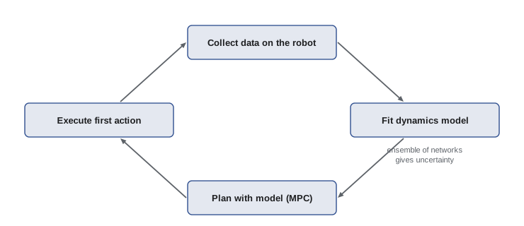
The danger is model error. A planner will find and exploit any place where the model is wrong in its favor, such as a predicted shortcut through a wall that does not exist in reality. Practical systems reduce this by keeping planning horizons short, re-planning at every step, training an ensemble of models and treating their disagreement as uncertainty to be avoided, and collecting more data in exactly the places where the model is uncertain. Learned world models, which predict future observations from images, extend these ideas to high-dimensional inputs and return in lesson 10.
| Approach | Data efficiency | Main risk | Example robot use |
|---|---|---|---|
| Model-free RL | Low: needs many interactions | Unsafe exploration, long training | Locomotion trained in simulation |
| Model-based RL with MPC | High: model reused many times | Planner exploits model errors | Learning to push or throw objects from a few hundred trials |
| Classical model plus control | No learning data needed | Model must be accurate | Industrial arms with LQR or computed torque |
| Hybrid: model plus learned residual | High | Residual may not generalize | Insertion with a learned friction correction |
Worked problem
Planning budget for sampling MPC
A robot runs MPC at 10 Hz with a learned model that takes 0.05 ms per one-step prediction on a GPU when batched. Each plan evaluates \( N \) candidate sequences of 15 steps across an ensemble of 5 models. What is the largest \( N \) that fits in 60 % of the control period?
Show solution
- Time available: \( 0.6 \times 100 \) ms = 60 ms.
- Predictions per candidate: \( 15 \times 5 = 75 \), costing \( 75 \times 0.05 = 3.75 \) ms if done one at a time.
- Batched on a GPU, assume candidates run in parallel in groups of 256 with the same per-step cost, so each group of 256 takes 3.75 ms.
- \( 60 / 3.75 = 16 \) groups, so \( N \approx 16 \times 256 = 4096 \).
Answer: About 4,000 candidate sequences per plan under these assumptions. Without batching, only 16 would fit, which shows why parallel hardware matters for sampling MPC.
When dynamic programming is enough
For many industrial problems, dynamic programming in one of its forms is the complete answer. Grid-based path planners in ROB-350, such as Dijkstra and A*, are dynamic programming on deterministic graphs. LQR and its nonlinear extensions handle balancing and trajectory tracking. Discrete scheduling problems, such as choosing the order of picks in a bin, can often be solved exactly. The lessons that follow assume you reach for learning only when the model is unknown, too expensive or too inaccurate, and they repeatedly borrow dynamic programming ideas: Bellman backups, generalized policy iteration and planning with models.
Common mistakes
MistakeExpecting value iteration to scale to a robot's continuous state.
InsteadUse function approximation, exploit structure such as LQR, or plan locally with MPC.
MistakeForgetting that value iteration needs a known model.
InsteadWithout a model, estimate values from experience (model-free) or learn a model first (model-based).
MistakePlanning long horizons with an imperfect learned model.
InsteadKeep horizons short, re-plan every step and penalize regions where an ensemble disagrees.
MistakeUsing RL for a near-linear system with a quadratic objective.
InsteadSolve it with LQR, which is optimal and needs no training data.
MistakeStopping value iteration after a fixed small number of sweeps.
InsteadCheck the largest change per sweep against a tolerance; distant states need many sweeps.
Summary and key terms
- Dynamic programming solves an MDP by computation when the model is known.
- Value iteration applies Bellman optimality backups until values converge; information spreads one step per sweep.
- Policy iteration alternates exact evaluation and greedy improvement and terminates in few iterations.
- Generalized policy iteration, interleaving partial evaluation and improvement, underlies most RL algorithms.
- Tabular methods suffer the curse of dimensionality; escapes are structure, function approximation and local planning.
- LQR is dynamic programming with a quadratic value function, and the Riccati recursion is value iteration.
- Model-based RL learns a dynamics model and plans with it, gaining data efficiency at the risk of exploiting model errors.
- Dynamic programming
- Solving sequential decision problems by breaking them into recursive subproblems using a known model.
- Bellman backup
- One application of a Bellman equation to update the value of a state.
- Value iteration
- Repeated Bellman optimality backups over all states until convergence.
- Policy iteration
- Alternating full policy evaluation and greedy policy improvement.
- Generalized policy iteration
- Any interleaving of partial policy evaluation and policy improvement.
- Curse of dimensionality
- The exponential growth of the state space as dimensions are added.
- Riccati equation
- The matrix recursion that gives the quadratic value function in LQR.
- Model-based RL
- Reinforcement learning that learns and uses a model of the dynamics.
- Model-predictive control
- Repeatedly optimizing a short-horizon plan with a model and executing its first action.
- Model ensemble
- Several learned models whose disagreement is used as a measure of uncertainty.
Practice problems
Work each problem on paper first, then reveal the answer to check.
Why does value iteration converge when \( \gamma < 1 \)?
Show answer
Each backup is a contraction that shrinks the error by at least a factor of \( \gamma \).
After three sweeps from zero, which states have useful values in a grid with one goal?
Show answer
States within about three steps of the goal.
What two steps does policy iteration alternate?
Show answer
Policy evaluation and greedy policy improvement.
A 6-dimensional state discretized into 10 values per dimension has how many states?
Show answer
\( 10^6 \), one million.
What form does the optimal value function take in LQR?
Show answer
Quadratic, \( V(x) = x^\top P x \).
What is the optimal LQR action?
Show answer
Linear feedback \( u = -Kx \).
Give one way to protect MPC from model errors.
Show answer
Short horizons, re-planning every step, or ensembles with uncertainty penalties.
Why is model-based RL attractive for real robots?
Show answer
A model can be reused many times, so fewer physical interactions are needed.
Name an everyday planner that is dynamic programming on a graph.
Show answer
Dijkstra's algorithm or A*.
What is a critic in actor-critic methods, in dynamic programming terms?
Show answer
An approximate policy evaluation that the actor improves against.
Lesson quiz · 5 questions
Score 60% or more to complete this lesson.
Create a free account to save your progress, take quizzes and earn a certificate.