
SLS-214 · Lesson 10 of 12 · 21 min
Spreadsheet skills for sales
▶ Video coming soon A video version of this lesson is on the way.
Maya had used spreadsheets at Juniper & Pine to track her commission, but Grace's sheets were on another level. On October 30, after the forecast session, Maya asked how Grace built them so quickly. Grace opened a blank sheet. "Almost everything I do uses about a dozen functions and three habits," she said. "Let me show you on a small sample, and then you can use the same steps on your own data."
This lesson covers the spreadsheet skills sales analysis needs most: laying out data properly, the functions that summarize it by condition, looking values up, pivot tables, moving averages and charts. The examples use common spreadsheet functions that work the same way, with minor differences, in Microsoft Excel and Google Sheets. Formulas are shown as plain text in tables.
Habit 1: one row per record, one column per field
Analysis is easy when data is laid out as a table: one row for each record, such as each opportunity, one column for each field, such as owner or stage, and one header row at the top. It is hard when data is laid out for reading, with merged cells, subtotals in the middle and several values crammed into one cell. A CRM export is usually already a clean table; the work is to keep it that way.
| A: Opportunity | B: Owner | C: Segment | D: Stage | E: First-year value | F: Close date | |
|---|---|---|---|---|---|---|
| 2 | Grainline Fabrication | Kevin | Manufacturer | Negotiate | 42,000 | 2026-11-27 |
| 3 | Southview Medical | Lisa | Clinic | Propose | 18,500 | 2026-11-20 |
| 4 | Carver Insurance | Nadia | Professional services | Propose | 12,600 | 2026-12-15 |
| 5 | Riverside School | Andrew | School | Discover | 9,800 | 2026-11-30 |
| 6 | Parkdale Clinic | Kevin | Clinic | Propose | 15,200 | 2026-11-24 |
| 7 | Holm & Pike LLP | Sam | Professional services | Negotiate | 22,400 | 2026-11-26 |
| 8 | Prairie Steel Works | Lisa | Manufacturer | Qualify | 31,000 | 2027-01-20 |
| 9 | Elm Street Dental | Nadia | Clinic | Negotiate | 7,900 | 2026-11-19 |
Two details matter. Values should be stored as numbers, without the word "dollars" or thousands separators typed in as text, so that they can be added; formatting can show the separators. Dates should be stored as real dates, so that they can be compared and subtracted. The ISO format, year-month-day, sorts correctly and is unambiguous in both Canada and the United States, where 11/12 can mean two different days.
Most spreadsheets can turn a range into a formal table (Format as Table in Excel, or Convert to table in Google Sheets). Formal tables extend formulas automatically as rows are added and let formulas refer to columns by name.
Habit 2: never type a number you can calculate
Every total, rate and forecast should be a formula that refers to the data, not a number typed in. Then, when the data changes, every result updates. Inputs that are assumptions, such as stage probabilities or a commission rate, should sit in their own clearly labeled cells, and formulas should refer to those cells. Grace's sheets kept assumptions on a separate tab called Settings.
When a formula is copied down a column, its references move with it: a formula in row 2 that refers to E2 becomes E3 in row 3. That is usually what you want. When a formula must keep pointing at the same cell, such as a commission rate in Settings, use an absolute reference, which most spreadsheets mark by placing a dollar sign before the column letter and the row number. Grace preferred to give such cells a name, such as CommissionRate, which is easier to read and never moves.
Habit 3: check the result another way
Grace checked every important number with a second method: a total by owner should add up to the grand total, a pivot table should agree with a SUMIFS formula, and a rate should be roughly what a mental estimate suggests. Spreadsheet errors are common, and most are caught by a simple cross-check.
Summarizing by condition
The functions sales analysts use most add, count or average only the rows that meet a condition.
| Question | Formula | Result |
|---|---|---|
| Total first-year value of Kevin's opportunities | =SUMIFS(E2:E9, B2:B9, "Kevin") | 57,200 |
| Number of opportunities in Negotiate | =COUNTIFS(D2:D9, "Negotiate") | 3 |
| Total value in Propose | =SUMIFS(E2:E9, D2:D9, "Propose") | 46,300 |
| Total value closing by November 30 | =SUMIFS(E2:E9, F2:F9, "<="&DATE(2026,11,30)) | 115,800 |
| Average value of clinic opportunities | =AVERAGEIFS(E2:E9, C2:C9, "Clinic") | 13,866.67 |
| Clinic value in Negotiate | =SUMIFS(E2:E9, C2:C9, "Clinic", D2:D9, "Negotiate") | 7,900 |
The pattern is always the same: the range to add or average comes first, then pairs of a range to test and the condition to test it against. SUMIFS and COUNTIFS accept several pairs, which act like "and": the last row of the table adds only rows that are both clinics and in Negotiate. Conditions can be text, numbers or comparisons such as "<=" joined to a date with the & symbol.
Worked problem
Checking a conditional total by hand
Check the result of =SUMIFS(E2:E9, F2:F9, "<="&DATE(2026,11,30)) from the table.
Show solution
- Find the rows with a close date on or before November 30, 2026: rows 2, 3, 5, 6, 7 and 9. Rows 4 and 8 close later.
- \[42{,}000 + 18{,}500 + 9{,}800 + 15{,}200 + 22{,}400 + 7{,}900 = 115{,}800\]
Answer: The formula is right: 115,800 dollars of first-year value in the sample is expected to close by November 30.
Looking values up
Lookup functions find a value in one table and bring it into another. Grace used them to attach a stage probability to each opportunity from the Settings tab.
| Settings: stage | Settings: probability |
|---|---|
| Qualify | 0.10 |
| Discover | 0.25 |
| Propose | 0.50 |
| Negotiate | 0.75 |
In a new column G, the formula =XLOOKUP(D2, Stages, Probs) finds the stage in D2 within the Stages column and returns the matching probability. Copied down, it fills in a probability for every row. Older spreadsheets use VLOOKUP or INDEX with MATCH for the same job; XLOOKUP is simpler and is available in current versions of Excel and in Google Sheets. A weighted value in column H is then =E2*G2.
Worked problem
Weighted value of the deals closing this quarter
Using the probabilities above, calculate the weighted first-year value of the six sample opportunities closing by November 30. In a spreadsheet this is =SUMPRODUCT((F2:F9<=DATE(2026,11,30))*E2:E9*G2:G9).
Show solution
- Grainline: 42,000 × 0.75 = 31,500.
- Southview: 18,500 × 0.50 = 9,250.
- Riverside: 9,800 × 0.25 = 2,450.
- Parkdale: 15,200 × 0.50 = 7,600.
- Holm & Pike: 22,400 × 0.75 = 16,800.
- Elm Street: 7,900 × 0.75 = 5,925.
- \[31{,}500 + 9{,}250 + 2{,}450 + 7{,}600 + 16{,}800 + 5{,}925 = 73{,}525\]
Answer: The weighted value closing by November 30 is 73,525 dollars. Inside SUMPRODUCT, the comparison gives 1 for rows that meet the date condition and 0 for those that do not, so the other rows drop out.
Pivot tables
A pivot table summarizes a table by one or more fields without writing formulas: drag Owner into rows, Stage into columns and First-year value into values, and the spreadsheet builds a grid of totals. Pivot tables are the fastest way to explore data, because the layout can be changed in seconds.
| Owner | Qualify | Discover | Propose | Negotiate | Total |
|---|---|---|---|---|---|
| Andrew | 9,800 | 9,800 | |||
| Kevin | 15,200 | 42,000 | 57,200 | ||
| Lisa | 31,000 | 18,500 | 49,500 | ||
| Nadia | 12,600 | 7,900 | 20,500 | ||
| Sam | 22,400 | 22,400 | |||
| Total | 31,000 | 9,800 | 46,300 | 72,300 | 159,400 |
Grace's cross-check: Kevin's row total, 57,200, matches the SUMIFS result above, and the Propose column, 46,300, matches the other SUMIFS. Pivot tables do not update automatically in every spreadsheet when the data changes; they may need to be refreshed, which is a common source of stale numbers in sales meetings.
Filters, sorting and data validation
Filters hide rows that do not meet a condition, which is useful for looking but dangerous for totals: some functions still include hidden rows. The SUBTOTAL function, or AGGREGATE in Excel, adds only visible rows. Sorting puts rows in order, for example by close date to see what is due this week. Data validation restricts what can be typed into a cell, such as a drop-down list of the five valid stages, which prevents the misspelled stage names that break SUMIFS conditions.
Moving averages
Monthly bookings jump around, which makes trends hard to see. A moving average smooths them by averaging each month with the months just before it. A three-month moving average for August averages June, July and August.
Worked problem
A three-month moving average
Ridgeline's team booked 214,000 dollars in June, 168,000 in July, 209,000 in August, 236,000 in September and 241,000 in October. Calculate the three-month moving average for August, September and October.
Show solution
- August: average June, July and August.
- \[\frac{214{,}000 + 168{,}000 + 209{,}000}{3} = 197{,}000\]
- September: average July, August and September.
- \[\frac{168{,}000 + 209{,}000 + 236{,}000}{3} \approx 204{,}333\]
- October: average August, September and October.
- \[\frac{209{,}000 + 236{,}000 + 241{,}000}{3} \approx 228{,}667\]
- In a spreadsheet with months in column A and bookings in column B, the August average in row 4 is =AVERAGE(B2:B4), copied down.
Answer: The moving average rose from 197,000 to about 204,333 and then about 228,667 dollars, a clearer upward trend than the jumpy monthly figures.
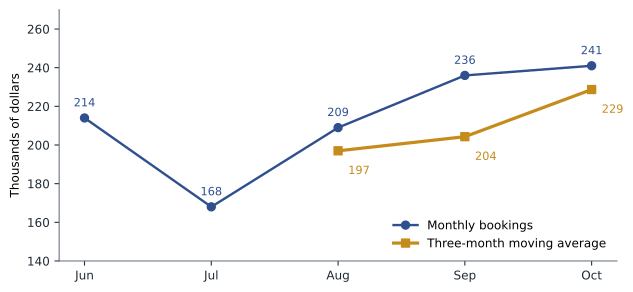
Moving averages lag behind turning points, because they include older months. They are good for seeing a trend and poor at spotting a sudden change. A three-month average is common for monthly sales; a longer window smooths more and lags more. The June to August figures add up to 591,000 dollars, the third-quarter total from earlier lessons, which is the kind of cross-check Grace liked.
Charts
A chart should answer one question. Grace's rules were short: use a bar chart to compare categories such as sellers or segments; a line chart for a trend over time; a stacked bar for parts of a total, such as booked plus weighted pipeline; and avoid pie charts with more than three or four slices and anything three-dimensional. Start bar charts at zero, label axes with units, and put the takeaway in the title, such as "Clinic win rate is above the team's". Lesson 11 builds these into dashboards.
Building a weekly pipeline sheet
Grace showed Maya the simple workflow she used every Friday. First, export open opportunities from the CRM with the same columns every week, so that formulas keep working. Second, paste the export into a Data tab, replacing last week's rows, and refresh any pivot tables. Third, let a Summary tab calculate everything else: totals by stage with SUMIFS, the weighted forecast with SUMPRODUCT, coverage by dividing by the quota on the Settings tab, and a short list of slipped deals using a filter on close dates earlier than today. The whole routine took about ten minutes once the sheet was built.
She also kept last week's export in a separate tab. Comparing the two showed what had changed: new opportunities, deals that had moved stage, deals whose amount or close date had changed, and deals that had closed. Most of the questions in Friday's forecast call came from that comparison. A sheet that shows only this week's numbers shows where the team is; a sheet that compares two weeks shows where it is going.
Spreadsheets also need protecting from accidents. Grace locked the formula cells on the Summary tab so that a stray keystroke could not overwrite them, kept a dated copy of each Friday's file, and wrote a one-line note at the top of each tab explaining what it held. When Maya took over part of the routine in December, those notes were what let her use the sheet without asking how it worked.
Common mistakes
MistakeTyping totals instead of using formulas.
InsteadCalculate every result from the data so it updates when the data changes.
MistakeStoring values or dates as text.
InsteadStore numbers as numbers and dates as dates; use formatting for display.
MistakeHard-coding assumptions inside formulas.
InsteadKeep assumptions in labeled or named cells on a Settings tab.
MistakeAdding filtered data with SUM.
InsteadUse SUBTOTAL or AGGREGATE, which ignore hidden rows.
MistakeTrusting a pivot table without refreshing it.
InsteadRefresh after the data changes, and cross-check it against a formula.
Summary and key terms
- Good sales spreadsheets follow three habits: one row per record and one column per field; never type a number that can be calculated; and check results another way.
- SUMIFS, COUNTIFS and AVERAGEIFS summarize rows that meet conditions; in the sample, Kevin's opportunities totaled 57,200 dollars and 115,800 dollars closed by November 30.
- XLOOKUP attaches values such as stage probabilities from a settings table, and SUMPRODUCT combines them into a weighted total of 73,525 dollars.
- Pivot tables summarize quickly but must be refreshed.
- Filters, sorting and data validation keep data usable.
- A three-month moving average smooths monthly bookings: 197,000, about 204,333 and about 228,667 dollars.
- Charts should answer one question each.
- Table
- Data laid out with one header row, one row per record and one column per field.
- SUMIFS
- A function that adds the values in rows meeting one or more conditions.
- XLOOKUP
- A function that finds a value in one range and returns the matching value from another.
- Pivot table
- A tool that summarizes a table by fields chosen by dragging, without formulas.
- Absolute reference
- A cell reference that does not change when a formula is copied.
- Moving average
- The average of a value over the latest few periods, recalculated each period to smooth fluctuations.
- Data validation
- A rule that limits what can be entered in a cell, such as a list of valid stages.
Practice problems
Work each problem on paper first, then reveal the answer to check.
Write a formula to count the opportunities owned by Lisa in the sample.
Show answer
=COUNTIFS(B2:B9, "Lisa"), which returns 2.
Monthly bookings were 100, 130 and 160 thousand dollars. What is the three-month moving average?
Show answer
(100 + 130 + 160) ÷ 3 = 130 thousand dollars.
Why should a stage be chosen from a drop-down list rather than typed?
Show answer
Misspelled stage names would be missed by conditions such as SUMIFS(..., "Propose").
Lesson quiz · 5 questions
Score 60% or more to complete this lesson.
Create a free account to save your progress, take quizzes and earn a certificate.