
PMP-130 · Lesson 8 of 12 · 28 min
Schedule compression, resource optimization and the schedule baseline
A first-pass schedule rarely satisfies everyone. It may finish later than a required date, overload some resources while leaving others idle, or rest on optimistic assumptions about uncertainty. This lesson covers the tools used to turn a first-pass schedule into one that can be approved as the baseline: crashing and fast tracking to compress the schedule, resource levelling and smoothing to make it feasible with available resources, Monte Carlo simulation to understand schedule risk, and the presentation formats and approval of the schedule baseline. It ends with release planning for adaptive work.
Schedule compression
Schedule compression shortens the schedule duration without reducing scope. The two techniques are crashing and fast tracking. Both work only on critical activities, because shortening a non-critical activity does not shorten the project. Both have costs: crashing adds money, fast tracking adds risk.
| Technique | How it works | Main cost | Example |
|---|---|---|---|
| Crashing | Adds resources to critical activities to shorten them (overtime, extra crews, faster delivery) | Higher direct cost; possible quality and fatigue effects | Paying the HVAC contractor for a second crew |
| Fast tracking | Performs activities in parallel or overlapping that were planned in sequence | Higher risk of rework; more coordination | Starting finishes in one zone while HVAC work continues in another |
Fast tracking is possible only where dependencies are discretionary or where partial overlap is genuinely safe. You cannot fast track a mandatory dependency such as obtaining a permit before demolition. Crashing works only where adding resources actually shortens the activity; it will not help a permit review by a city department.
Crashing decisions use cost slope, the extra cost per unit of time saved:
The rule is to crash the critical activity with the lowest cost slope first, one period at a time, recalculating the critical path after each step because the critical path can change. Stop when the target is reached, when no further crashing is possible, or when the cost exceeds the benefit (for example, the daily cost of delay or the value of finishing earlier).
# Crashing the Project Compass fit-out: cheapest days first (invented costs)
acts = {  # id: (normal days, crash days, crash cost per day saved)
    "A": (15, 12, 900), "B": (20, 20, 0), "C": (30, 24, 400), "D": (10, 8, 1500),
    "E": (15, 12, 700), "F": (20, 16, 1200), "G": (15, 12, 1000),
    "H": (10, 8, 1800), "I": (10, 8, 300), "J": (8, 6, 2500), "K": (2, 2, 0),
}
pred = {"A": [], "B": ["A"], "C": ["A"], "D": ["B"], "E": ["D"], "F": ["D"],
        "G": ["E", "F"], "H": ["C", "G"], "I": ["C"], "J": ["H"], "K": ["I", "J"]}
order = list("ABCDEFGHIJK")

def cpm(dur):
    ef = {}
    for a in order:
        ef[a] = max((ef[p] for p in pred[a]), default=0) + dur[a]
    end = max(ef.values())
    ls = {}
    for a in reversed(order):
        lf = min((ls[s] for s in order if a in pred[s]), default=end)
        ls[a] = lf - dur[a]
    crit = {a for a in order if ls[a] == ef[a] - dur[a]}
    return end, crit

dur = {a: v[0] for a, v in acts.items()}
target, spent = 85, 0
end, crit = cpm(dur)
print(f"Normal duration {end} days")
while end > target:
    options = [a for a in crit if dur[a] > acts[a][1]]
    if not options:
        print("No single activity left to crash"); break
    a = min(options, key=lambda x: acts[x][2])
    dur[a] -= 1; spent += acts[a][2]
    new_end, crit = cpm(dur)
    print(f"Crash {a} by 1 day at ${acts[a][2]:,}: duration {new_end}, crashing cost ${spent:,}")
    end = new_end
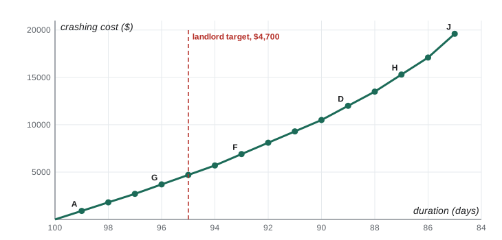
print("Critical path now:", "-".join(a for a in order if a in crit))Normal duration 100 days Crash A by 1 day at $900: duration 99, crashing cost $900 Crash A by 1 day at $900: duration 98, crashing cost $1,800 Crash A by 1 day at $900: duration 97, crashing cost $2,700 Crash G by 1 day at $1,000: duration 96, crashing cost $3,700 Crash G by 1 day at $1,000: duration 95, crashing cost $4,700 Crash G by 1 day at $1,000: duration 94, crashing cost $5,700 Crash F by 1 day at $1,200: duration 93, crashing cost $6,900 Crash F by 1 day at $1,200: duration 92, crashing cost $8,100 Crash F by 1 day at $1,200: duration 91, crashing cost $9,300 Crash F by 1 day at $1,200: duration 90, crashing cost $10,500 Crash D by 1 day at $1,500: duration 89, crashing cost $12,000 Crash D by 1 day at $1,500: duration 88, crashing cost $13,500 Crash H by 1 day at $1,800: duration 87, crashing cost $15,300 Crash H by 1 day at $1,800: duration 86, crashing cost $17,100 Crash J by 1 day at $2,500: duration 85, crashing cost $19,600 Critical path now: A-B-D-F-G-H-J-K
To meet a landlord target of day 95, the team crashes design (A) by 3 days at $900 a day and finishes (G) by 2 days at $1,000 a day, for $4,700. Going further, to 85 days, costs $19,600 in total, with each extra day more expensive than the last. Two observations are typical. First, A was crashed before cheaper activities like C ($400 a day) and I ($300 a day) because those are not critical. Second, by the end, several paths are almost equally long; the schedule has become fragile, with little float anywhere. A compressed schedule is a riskier schedule, which the sponsor should understand before approving it.
Fast tracking for Project Compass might mean starting the electrical rough-in (E) and HVAC upgrade (F) in different zones as soon as each zone's demolition is complete, rather than waiting for all demolition to finish. That creates leads, and it requires careful coordination of trades and inspections. If drawings are not final, fast tracking design and construction risks expensive rework. As a rule, fast track first when risk is acceptable because it costs less money; crash when money is cheaper than risk.
Resource optimization
A schedule that ignores resource limits may be impossible to execute. Resource optimization adjusts the schedule so that resource demand fits supply. A resource histogram, a bar chart of resource demand over time, makes overallocation visible.
Resource levelling adjusts start and finish dates based on resource constraints, with the goal of balancing demand with available supply. It is used when resources are available only at certain times or in limited quantities, or are overallocated. Levelling can change the critical path and often extends the project duration. Resource smoothing adjusts activities so that resource demand stays within predefined limits, but only within their float; it does not change the critical path or the finish date, and as a result it may not remove every overallocation.
# Electricians needed per week on the fit-out: smoothing versus a resource-limited plan (invented data)
crew = 4                                      # electricians the contractor can supply
float_weeks = 1                               # total float on data cabling (part of E)
base = {  # activity: (start week, end week, electricians per week)
    "Electrical rough-in": (10, 12, 2),
    "HVAC controls wiring": (10, 13, 2),
    "Data cabling": (11, 12, 2),
    "Kiosk and gate power": (17, 18, 2),
}

def histogram(plan):
    return {w: sum(n for s, e, n in plan.values() if s <= w <= e) for w in range(10, 19)}

def show(title, plan):
    h = histogram(plan)
    print(title)
    print("  week: " + " ".join(f"{w:2d}" for w in h))
    print("  need: " + " ".join(f"{n:2d}" for n in h.values()))
    over = [w for w, n in h.items() if n > crew]
    print(f"  peak {max(h.values())}, weeks over {crew}: {over if over else 'none'}")

def shifted(plan, act, weeks):
    s, e, n = plan[act]
    p = dict(plan); p[act] = (s + weeks, e + weeks, n)
    return p

show("Original plan:", base)
smooth = shifted(base, "Data cabling", float_weeks)
show("Smoothing: move cabling within its 1 week of float", smooth)
limited = shifted(base, "Data cabling", 2)
show("Resource-limited: move cabling 2 weeks", limited)
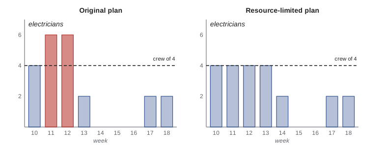
print(f"The resource-limited plan uses {2 - float_weeks} week beyond the float, so the finish moves 1 week later")Original plan: week: 10 11 12 13 14 15 16 17 18 need: 4 6 6 2 0 0 0 2 2 peak 6, weeks over 4: [11, 12] Smoothing: move cabling within its 1 week of float week: 10 11 12 13 14 15 16 17 18 need: 4 4 6 4 0 0 0 2 2 peak 6, weeks over 4: [12] Resource-limited: move cabling 2 weeks week: 10 11 12 13 14 15 16 17 18 need: 4 4 4 4 2 0 0 2 2 peak 4, weeks over 4: none The resource-limited plan uses 1 week beyond the float, so the finish moves 1 week later
The contractor can supply four electricians. The original plan needs six in weeks 11 and 12 because data cabling overlaps the rough-in and HVAC controls wiring. Smoothing moves data cabling one week later, within its float, which fixes week 11 but not week 12. Levelling moves it two weeks, removing all overallocation, but that uses one week more than the float available, so the finish moves one week later. The project manager now has a real choice: accept the later finish, pay for two more electricians in week 12 (crashing), or split the data cabling work. Which option is right depends on the cost of delay and the contractor's options.
Exam questions often hinge on the difference. If the question says the finish date cannot move, the answer is smoothing (or another technique such as adding resources). If the question describes a resource that is available only part time or a fixed crew, and accepts that the date may move, levelling is the answer.
Monte Carlo simulation and schedule risk
The critical path calculation uses single durations. Lesson 6 added three-point estimates to a single path. But in a real network, uncertainty on several paths interacts. Where paths merge, the merge activity must wait for the latest of them, so uncertainty on near-critical paths pushes the expected finish later than the critical path alone suggests. This is called merge bias. Monte Carlo simulation handles it by running the schedule thousands of times, each time drawing a random duration for every activity from its distribution, and recording the finish. The result is a distribution of finish dates.
# Monte Carlo schedule risk for the Project Compass fit-out (triangular estimates)
import random, statistics
random.seed(130)
tri = {  # (optimistic, most likely, pessimistic) working days
    "A": (12, 15, 21), "B": (15, 20, 35), "C": (25, 30, 45), "D": (8, 10, 14),
    "E": (12, 15, 20), "F": (16, 20, 30), "G": (12, 15, 21), "H": (8, 10, 13),
    "I": (8, 10, 12), "J": (6, 8, 11), "K": (2, 2, 2),
}
pred = {"A": [], "B": ["A"], "C": ["A"], "D": ["B"], "E": ["D"], "F": ["D"],
        "G": ["E", "F"], "H": ["C", "G"], "I": ["C"], "J": ["H"], "K": ["I", "J"]}

def finish(d):
    ef = {}
    for a in "ABCDEFGHIJK":
        ef[a] = max((ef[p] for p in pred[a]), default=0) + d[a]
    return ef["K"]

runs = sorted(finish({a: random.triangular(o, p, m) for a, (o, m, p) in tri.items()})
              for _ in range(10000))
print(f"Deterministic (most likely) duration: {finish({a: v[1] for a, v in tri.items()})} days")
print(f"Mean of simulations: {statistics.mean(runs):.1f} days")
for pct in (50, 80, 90):
    print(f"P{pct}: {runs[int(len(runs) * pct / 100) - 1]:.1f} days")
for deadline in (95, 105, 110):
    p = sum(r <= deadline for r in runs) / len(runs)
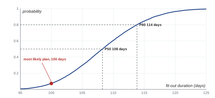
print(f"Chance of finishing within {deadline} days: {p:.0%}")Deterministic (most likely) duration: 100 days Mean of simulations: 108.6 days P50: 108.2 days P80: 113.8 days P90: 116.6 days Chance of finishing within 95 days: 0% Chance of finishing within 105 days: 30% Chance of finishing within 110 days: 61%
The most likely durations give 100 days. The simulation's median (P50) is about 108 days and its P80, the duration with an 80 % chance of not being exceeded, is about 114 days. There is effectively no chance of meeting 95 days without compression, about a 30 % chance of finishing within 105 days and about 61 % within 110. Compare this with the single-path PERT estimate in lesson 6, which suggested about 84 % within 109 days. The simulation is less optimistic for two reasons: triangular distributions give more weight to the tails than PERT's beta weighting, and the non-critical paths through C and E sometimes become critical in individual runs.
This is why many organizations set schedule reserves and commit to dates at a chosen confidence level, such as P80 for public announcements, while managing the team to a more aggressive internal target. For Project Compass, the project manager recommends announcing the soft opening as "mid-August" (about P80 for the fit-out plus the remaining work) while managing to the plan dates. Schedule risk analysis is covered further in PMP-131 alongside quantitative risk analysis.
Presenting the schedule
Different audiences need different views of the same schedule.
| Format | Shows | Best for |
|---|---|---|
| Milestone chart | Key milestones and their dates, with status | Sponsors, boards, executives |
| Bar (Gantt) chart | Activities as bars against a timeline, often with dependencies and float | Project team, coordination meetings |
| Network diagram | Logic and dependencies, critical path | Schedulers, analysing impact of changes |
| Summary (hammock) bars | Rolled-up groups of activities | Management reports |
| Release and iteration plans | Features or goals per release and sprint | Adaptive teams and product stakeholders |
The schedule model is the underlying set of activities, durations, logic, resources and calendars, usually held in scheduling software. The schedule presentations are outputs from it. Keeping one model and producing views from it avoids inconsistent versions.
The schedule baseline
The schedule baseline is the approved version of the schedule model, with baseline start and finish dates. It is approved by the appropriate stakeholders, typically the sponsor and, for contracted work, may be referenced in agreements. Once approved, actual progress is compared against it to calculate variances. It changes only through change control.
Before approval, the project manager should check that the schedule is realistic: logic complete and sound, durations based on estimates with a documented basis, resources levelled or smoothed, risks reflected in reserves, and key stakeholders consulted. A schedule that is approved but not believed by the team is not a baseline; it is a wish.
Worked problem
Choosing between compression and scope change
Project Compass's board asks for the soft opening two weeks earlier than planned, to coincide with a community festival. The crashing analysis shows two weeks (10 working days) would cost about $10,500 and leave the schedule with almost no float. Fast tracking finishes with HVAC work is possible in two zones but risks rework if HVAC ducts need to move. What should the project manager present?
Show solution
- Quantify options: crash for about $10,500; fast track with a risk of rework; or a partial opening with the children's area finished first.
- Explain risk: the compressed schedule has little float, so any slip delays the festival date.
- Consider scope options: open with a smaller collection and complete tagging after opening.
- Recommend: a modest combination, such as fast tracking in one zone plus a partial opening, with clear risks and costs.
Answer: Present options with their costs and risks and let the board decide. The project manager's job is to inform the trade-off, not simply to say yes or no.
Release planning in adaptive work
Adaptive projects build schedules differently. A release plan shows which features are expected in which release, based on velocity or throughput forecasts. Each iteration has a fixed length, and the team plans its content at the start. Forecasts are updated each iteration as velocity becomes clearer. Instead of a critical path, the risk is that the backlog grows or velocity falls; burn-up and burndown charts make both visible. In Project Compass, release 1 of the app must be in the app stores before the soft opening, so its release plan becomes an interface milestone in the fit-out schedule.
Common mistakes
MistakeCrashing or fast tracking non-critical activities.
InsteadCompress only critical activities; recalculate after each change.
MistakeFast tracking mandatory dependencies.
InsteadOverlap only discretionary dependencies or work that can safely proceed in parallel.
MistakeUsing levelling when the finish date must not move.
InsteadUse smoothing within float, or add resources, if the date is fixed.
MistakeAnnouncing the deterministic finish date as a commitment.
InsteadUse risk analysis to choose a date with an acceptable confidence level.
MistakeApproving a schedule the team does not believe.
InsteadBuild the baseline with the team, based on documented estimates and resource limits.
Summary and key terms
- Crashing adds resources to critical activities; choose the lowest cost slope first and recalculate.
- Fast tracking overlaps activities; it adds risk and works only for discretionary or safe overlaps.
- Resource levelling resolves overallocation and may extend the schedule; smoothing stays within float.
- Monte Carlo simulation shows the range of likely finishes and captures merge bias.
- Commit to dates at a stated confidence level, such as P80.
- Milestone charts suit executives; Gantt charts suit teams; network diagrams show logic.
- The schedule baseline is the approved schedule model, changed only through change control.
- Schedule compression
- Techniques to shorten schedule duration without reducing scope.
- Crashing
- Shortening duration by adding resources to critical activities.
- Fast tracking
- Performing activities in parallel that were planned in sequence.
- Cost slope
- The additional cost per unit of time saved by crashing an activity.
- Resource levelling
- Adjusting dates to balance resource demand with supply, possibly changing the critical path.
- Resource smoothing
- Adjusting activities within their float to keep resource demand within limits.
- Resource histogram
- A bar chart showing resource demand over time.
- Monte Carlo simulation
- Running a model many times with random inputs to produce a distribution of outcomes.
- Merge bias
- The tendency of merging uncertain paths to push the expected finish later than any single path suggests.
- Schedule baseline
- The approved version of the schedule model used as a basis for comparison.
Practice problems
Work each problem on paper first, then reveal the answer to check.
An activity can be shortened from 10 to 7 days for an extra $6,000. Cost slope?
Show answer
$6,000 / 3 = $2,000 per day.
Critical activities X ($1,500/day) and Y ($900/day) can be crashed. Which first?
Show answer
Y, the lower cost slope.
Which compression technique mainly adds risk rather than cost?
Show answer
Fast tracking.
Can a permit review by a city department be crashed by adding project staff?
Show answer
Usually not; the work is external and outside the project's control.
What did crashing Project Compass to day 95 cost?
Show answer
$4,700 (A by 3 days, G by 2 days).
The finish date is fixed and a resource is overallocated. Which technique?
Show answer
Resource smoothing, or adding resources, rather than levelling.
What does P80 mean?
Show answer
The duration or cost with an 80 % probability of not being exceeded.
Why was the simulated P50 later than 100 days?
Show answer
Skewed estimates and merge bias where uncertain paths join.
Which schedule format suits a board meeting?
Show answer
A milestone chart.
How does an adaptive team forecast a release date?
Show answer
Using remaining backlog and measured velocity or throughput, updated each iteration.
Lesson quiz · 5 questions
Score 60% or more to complete this lesson.
Create a free account to save your progress, take quizzes and earn a certificate.