
ROB-220 · Lesson 7 of 12 · 31 min
Localization sensors: GNSS, RTK, UWB and odometry
A robot that works outdoors, or across a large building, needs to know where it is in a global frame: on a farm field, along a road, in a warehouse aisle. Some sensors measure that directly. Satellite navigation gives position anywhere with a clear view of the sky; real-time kinematic corrections sharpen it to centimetres; ultra-wideband radio beacons do a similar job indoors; and wheel odometry, visual odometry and the IMU fill the gaps between absolute fixes. This lesson covers the sensors and their error behaviour. How their measurements are combined into a single best estimate is the subject of ROB-310 and ROB-340.
How GNSS works
Global navigation satellite systems (GNSS) include the American GPS, the European Galileo, Russia's GLONASS and China's BeiDou, with more than 100 satellites in orbit between them. Each satellite broadcasts its precise orbit and a timing signal derived from atomic clocks. A receiver measures the apparent travel time of each signal, multiplies by the speed of light to get a pseudorange, and solves for its own position and its clock error. Four unknowns (x, y, z and receiver clock offset) need at least four satellites; more satellites improve accuracy and robustness, which is why multi-constellation receivers that track all four systems have become standard.
Here \( \rho_i \) is the pseudorange to satellite i, \( \mathbf{s}_i \) its position, \( \mathbf{x} \) the receiver position, \( \delta t \) the receiver clock error and \( \varepsilon_i \) everything else. That everything else is substantial: the ionosphere and troposphere delay the signals, satellite clock and orbit errors remain, signals reflect off buildings before arriving (multipath), and receiver noise adds a little. A standalone consumer receiver with a clear sky typically achieves a few metres horizontally, and much worse among tall buildings, under trees or near walls.
Dilution of precision and the error budget
The geometry of the visible satellites multiplies the ranging error. If all the satellites are clustered in one part of the sky, small range errors produce large position errors; if they are spread around the sky, the position is well constrained. This amplification is expressed as dilution of precision (DOP). Horizontal DOP (HDOP) of about 1 is excellent, 2 is good, and above 5 is poor. A useful rule of thumb is that the horizontal position error is roughly HDOP times the user range error.
Worked problem
Position error in an urban canyon
A receiver has a user equivalent range error of 3 m. In an open field its HDOP is 0.9; in a street lined with tall buildings, only a narrow strip of sky is visible and the HDOP rises to 4.5. Estimate the horizontal error in each case. What happens if multipath adds another 6 m of range error in the street?
Show solution
- Open field: \( 0.9 \times 3 = 2.7 \) m.
- Street, geometry only: \( 4.5 \times 3 = 13.5 \) m.
- Street with multipath: range error \( \sqrt{3^2 + 6^2} = 6.7 \) m, so \( 4.5 \times 6.7 \approx 30 \) m.
Answer: About 3 m in the open but roughly 14 m in the street, and around 30 m once multipath is included. Delivery robots on city sidewalks cannot rely on standalone GNSS.
Augmentation: SBAS, PPP and RTK
Several techniques remove most of the common errors. Satellite-based augmentation systems (SBAS) broadcast corrections from geostationary satellites; the North American system, WAAS, covers both Canada and the United States and brings accuracy to around 1 to 2 m, mainly for aviation. Precise point positioning (PPP) uses precise orbit and clock products to reach decimetre or centimetre accuracy with a single receiver, but traditionally needs many minutes to converge.
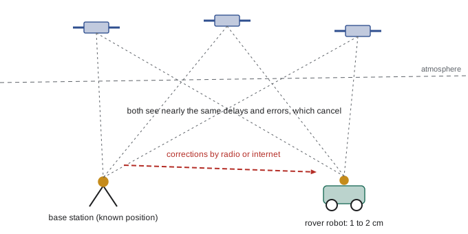
Real-time kinematic (RTK) positioning is the workhorse for robots that need centimetres. A base station at a precisely known position, either the robot owner's own or one in a network, tracks the same satellites as the robot's receiver (the rover) and sends corrections, usually over a radio link or the internet using the NTRIP protocol. Because base and rover see nearly the same atmospheric and satellite errors when they are within a few tens of kilometres, the differences cancel. RTK also uses the carrier phase of the signals, whose wavelength is about 19 cm for GPS L1, rather than just the code timing. Once the receiver has resolved the integer number of carrier wavelengths to each satellite, a fixed solution, it typically achieves about 1 to 2 cm horizontally. Before that, or when too few satellites are tracked, it reports a float solution at the decimetre level.
| Service | Who provides it | Typical accuracy | Notes |
|---|---|---|---|
| Standalone GNSS | Satellites only | A few metres | Degrades badly near buildings and trees |
| WAAS (SBAS) | Covers Canada and the US | About 1–2 m | Free; designed for aviation |
| CSRS-PPP | Natural Resources Canada | Centimetres (post-processed) | Free online processing of recorded data |
| Canadian Active Control System | Natural Resources Canada | Reference stations and products | Underpins the national reference frame |
| Provincial and commercial RTK networks | Provinces and private networks | 1–2 cm | Corrections over the internet (NTRIP), often by subscription |
| Own RTK base | The robot operator | 1–2 cm near the base | Needs a surveyed or self-surveyed base position |
Worked problem
How far from the base can a rover be?
An RTK receiver specifies 8 mm + 1 ppm horizontal accuracy. What is the expected error when the rover is 2 km, 15 km and 40 km from the base?
Show solution
- 1 ppm means 1 mm per kilometre of baseline.
- 2 km: \( 8 + 2 = 10 \) mm. 15 km: \( 8 + 15 = 23 \) mm.
- 40 km: \( 8 + 40 = 48 \) mm, and in practice fixing the integer ambiguities becomes slower and less reliable at this distance.
Answer: About 1 cm at 2 km, 2.3 cm at 15 km and nearly 5 cm at 40 km. Farms and construction sites usually keep the base within about 10 to 20 km.
GNSS position alone does not give heading for a slow or stationary robot. Dual-antenna receivers solve this by measuring the vector between two antennas a metre or so apart with RTK precision, giving heading accurate to a fraction of a degree, which is why agricultural autosteer systems often carry two antennas.
Ultra-wideband and other indoor beacons
Satellite signals do not penetrate buildings usefully, so indoor robots need other references. Ultra-wideband (UWB) radio sends very short pulses spread over a bandwidth of 500 MHz or more, which makes it possible to time the arrival of the direct path precisely and to tell it apart from reflections. Two UWB devices measure the distance between them by two-way ranging: one sends a message, the other replies after a known delay, and the round-trip time gives the range to about 10 cm. A robot that measures ranges to three or more fixed anchors at known positions can find its position by trilateration, much like GNSS. UWB is used for warehouse robot positioning, tracking people and tools in factories, and keeping lawn-mowing robots inside their boundaries without buried wire.
Worked problem
Two-way ranging and clock accuracy
A UWB tag measures a round-trip time of 233.40 ns, and the anchor's reply delay is 200.00 ns. What is the range? If the timing has an error of 0.5 ns, how big is the range error?
Show solution
- Time of flight both ways: \( 233.40 - 200.00 = 33.40 \) ns.
- Range: \( 3 \times 10^8 \times 33.40 \times 10^{-9}/2 = 5.01 \) m.
- Range error from 0.5 ns: \( 3 \times 10^8 \times 0.5 \times 10^{-9}/2 = 0.075 \) m.
Answer: About 5.0 m, and half a nanosecond of timing error means about 7.5 cm of range error. Precise timing, and correcting for clock drift during the reply delay, is the heart of UWB design.
Other indoor options include fiducial markers (printed tags such as AprilTags that a camera can locate precisely), reflectors used by laser-guided vehicles, magnetic tape or floor codes for automated guided vehicles, and Wi-Fi or Bluetooth signal strength, which is cheap but only accurate to metres. UWB is a radio transmitter and therefore needs certification; the same regulators named in lesson 5 set its power limits and permitted bands.
Wheel odometry and dead reckoning
Between absolute fixes, robots estimate motion from their own sensors, a process called dead reckoning. Wheel odometry integrates encoder readings (lesson 2) through the robot's kinematic model (ROB-210) to update position and heading. It is precise over short distances and available at high rates, but its errors accumulate without bound. Systematic errors include an incorrect wheel diameter, unequal wheel diameters and an incorrect track width; random errors include wheel slip, uneven floors and bumps. Heading errors are the most damaging, because each degree of heading error turns every subsequent metre of travel into sideways error.
Worked problem
Odometry drift from a wheel-diameter mismatch
A differential-drive robot with a track width of 0.40 m has a left wheel whose effective diameter is 0.5 % smaller than assumed. The robot drives what it believes is a straight 20 m line. What heading error and sideways drift result?
Show solution
- Distance difference between wheels: the left wheel travels 0.5 % less, so \( \Delta s = 0.005 \times 20 = 0.10 \) m.
- Heading change: \( \Delta\psi = \Delta s/b = 0.10/0.40 = 0.25 \) rad \( \approx 14.3° \).
- For a gentle arc, sideways drift is about \( L\,\Delta\psi/2 = 20 \times 0.25/2 = 2.5 \) m.
Answer: A heading error of about 14° and roughly 2.5 m of sideways drift over 20 m, all from a half-percent diameter difference such as uneven tyre wear or load. Calibrating wheel diameters and track width, for example with the UMBmark square-path test, is essential.
Visual odometry and lidar odometry estimate motion by tracking features or matching scans between successive frames; they do not slip on wet floors but drift slowly too and fail in featureless or dynamic scenes. Combining wheel odometry, an IMU and visual or lidar odometry, then correcting the result with absolute fixes from GNSS, UWB or map matching, is the standard architecture of modern robot localization. The sensors in this lesson are the inputs to that architecture; lesson 11 introduces the simplest way to combine them.
import numpy as np
# Dead reckoning with a small left-wheel scale error on a "straight" 20 m drive
b, ds, steps = 0.40, 0.01, 2000          # track width (m), step (m), 2000 steps = 20 m
scale_left = 0.995                        # left wheel 0.5 % small
x = y = th = 0.0
for _ in range(steps):
    dl, dr = ds * scale_left, ds          # true wheel travel when encoders say ds each
    d, dth = (dl + dr) / 2, (dr - dl) / b
    x += d * np.cos(th + dth / 2); y += d * np.sin(th + dth / 2); th += dth
print(f"robot believes: x = 20.00 m, y = 0.00 m, heading 0.0 deg")
print(f"actually at: x = {x:5.2f} m, y = {y:5.2f} m, heading {np.degrees(th):4.1f} deg")robot believes: x = 20.00 m, y = 0.00 m, heading 0.0 deg actually at: x = 19.74 m, y = 2.48 m, heading 14.3 deg
Common mistakes
MistakeExpecting standalone GNSS to give lane- or sidewalk-level position in a city.
InsteadMultipath and poor geometry give errors of tens of metres; use RTK, fusion with other sensors and map matching.
MistakeTreating an RTK float solution as centimetre-accurate.
InsteadOnly a fixed solution gives centimetres; check the solution status and fall back gracefully when it drops to float.
MistakePlacing an RTK base far from the work area.
InsteadError grows by about 1 mm per kilometre and ambiguity fixing degrades; keep baselines short.
MistakeAssuming GNSS gives heading when the robot is stationary.
InsteadHeading from successive positions needs motion; use dual antennas, a magnetometer or other sensors.
MistakeRunning wheel odometry with nominal wheel diameters and track width.
InsteadCalibrate them on the real robot and floor; half a percent of error causes metres of drift.
Summary and key terms
- GNSS receivers solve for position and clock offset from pseudoranges to at least four satellites.
- Atmospheric delays, clock and orbit errors and multipath give standalone accuracy of a few metres.
- Dilution of precision multiplies range errors; urban canyons can push errors to tens of metres.
- SBAS, PPP and RTK remove common errors; RTK fixed solutions reach 1–2 cm near a base.
- Dual-antenna receivers give heading; national agencies provide reference stations and correction services.
- UWB two-way ranging gives about 10 cm ranges indoors, and trilateration gives position.
- Wheel odometry drifts from diameter, track-width and slip errors and must be calibrated and fused.
- GNSS
- Global navigation satellite system, such as GPS, Galileo, GLONASS or BeiDou.
- Pseudorange
- A satellite range measurement that includes the receiver clock error.
- Dilution of precision
- The factor by which satellite geometry amplifies range errors.
- Multipath
- Signals reaching the receiver after reflecting off surfaces.
- SBAS
- Satellite-based augmentation system, such as WAAS.
- RTK
- Real-time kinematic positioning using corrections from a nearby base station.
- Fixed solution
- An RTK solution with resolved carrier-phase integers, accurate to centimetres.
- NTRIP
- A protocol for streaming GNSS corrections over the internet.
- Ultra-wideband
- Radio using very short pulses over a wide bandwidth, allowing precise ranging.
- Dead reckoning
- Estimating position by integrating measured motion from a known start.
Practice problems
Work each problem on paper first, then reveal the answer to check.
Why does a GNSS receiver need at least four satellites?
Show answer
To solve for three position coordinates and the receiver clock error.
A receiver has a range error of 2 m and HDOP 1.5. Estimate the horizontal error.
Show answer
About 3 m.
What is the wavelength of the GPS L1 carrier, roughly?
Show answer
About 19 cm.
An RTK spec is 10 mm + 1 ppm. What is the error 25 km from the base?
Show answer
35 mm.
What does a dual-antenna GNSS receiver add?
Show answer
Heading, from the precise vector between the two antennas.
A UWB round trip is 140 ns with a 100 ns reply delay. What is the range?
Show answer
\( 3 \times 10^8 \times 40 \times 10^{-9}/2 = 6 \) m.
How many anchors are needed for 2-D UWB trilateration without ambiguity?
Show answer
At least three.
A heading error of 2° persists over 100 m of travel. What is the sideways error?
Show answer
\( 100 \sin 2° \approx 3.5 \) m.
Name one systematic and one random source of odometry error.
Show answer
Systematic: wrong wheel diameter or track width. Random: wheel slip or bumps.
Why is visual odometry useful alongside wheel odometry?
Show answer
It does not suffer wheel slip, so its errors are largely independent.
Lesson quiz · 5 questions
Score 60% or more to complete this lesson.
Create a free account to save your progress, take quizzes and earn a certificate.