
ROB-230 · Lesson 10 of 12 · 33 min
Discrete-time systems and the z-transform
Inside a robot's controller there are no differential equations, only loops of code that run once per sample: read the sensors, update some variables, write the outputs. Such code implements a difference equation, the discrete-time counterpart of a differential equation, and its behaviour can be analysed with tools that parallel the continuous ones exactly. The z-transform plays the role of the Laplace transform, the unit delay \( z^{-1} \) plays the role of the integrator 1/s, the unit circle plays the role of the imaginary axis, and the inside of the circle plays the role of the left half-plane. This lesson builds that toolkit, then tackles the practical problem every embedded engineer faces: converting a continuous design, such as a filter or controller drawn in s, into code. Different conversion methods, forward Euler, backward Euler, Tustin and the matched exact method, have different accuracy and stability properties, and choosing badly can make a perfectly good design go unstable on the robot.
Difference equations
A linear time-invariant discrete system relates its current output to current and past inputs and past outputs:
This is directly code: keep the last few inputs and outputs in variables, and each sample compute the weighted sum. If all the a coefficients are zero the output depends only on inputs, the impulse response has finite length, and the system is an FIR filter, like the moving average of lesson 3. If any a is nonzero the output feeds back on itself, the impulse response goes on forever, and the system is recursive, or infinite impulse response (IIR). The first-order low-pass filter \( y[n] = \alpha y[n-1] + (1 - \alpha)x[n] \) used for sensor smoothing in ROB-220 is the simplest IIR system. Its impulse response is \( (1 - \alpha)\alpha^n \), which decays if \( |\alpha| < 1 \) and explodes if \( |\alpha| > 1 \).
Worked problem
Running a difference equation by hand
A filter is \( y[n] = 0.6\,y[n-1] + 0.4\,x[n] \), starting at rest. Find the first four outputs for a unit step input, and the final value.
Show solution
- y[0] = 0.4.
- y[1] = 0.6 × 0.4 + 0.4 = 0.64.
- y[2] = 0.6 × 0.64 + 0.4 = 0.784; y[3] = 0.6 × 0.784 + 0.4 = 0.870.
- Final value: set y[n] = y[n−1] = Y, so Y = 0.6Y + 0.4, giving Y = 1.
Answer: The outputs are 0.4, 0.64, 0.784, 0.870, approaching 1 geometrically: the remaining error shrinks by a factor of 0.6 each sample. Each sample of a recursive filter costs only two multiplications and one addition, which is why IIR filters are popular on small microcontrollers.
The z-transform
The z-transform of a sequence x[n] that is zero for n < 0 is
where z is a complex variable. It is the discrete analogue of the Laplace transform; in fact, for a sampled signal it equals the Laplace transform with the substitution \( z = e^{sT} \). Its key property is the delay rule: delaying a sequence by one sample multiplies its transform by \( z^{-1} \),
so \( z^{-1} \) is the unit delay, the memory element of digital systems, drawn as a block in digital filter diagrams. Applying the transform to the general difference equation with zero initial conditions gives the discrete transfer function
which can be read straight off the code and vice versa. A few transform pairs suffice for most work: the unit impulse \( \delta[n] \) transforms to 1, the unit step to \( z/(z - 1) \), and the geometric sequence \( a^n \) to \( z/(z - a) \). Convolution of sequences becomes multiplication of transforms, as in continuous time.
Worked problem
Transfer function of a smoothing filter
Find the transfer function, pole and DC gain of \( y[n] = 0.6\,y[n-1] + 0.4\,x[n] \).
Show solution
- Transform: \( Y = 0.6z^{-1}Y + 0.4X \).
- \( H(z) = \dfrac{0.4}{1 - 0.6z^{-1}} = \dfrac{0.4z}{z - 0.6} \).
- Pole at z = 0.6.
- DC corresponds to z = 1 (since \( z = e^{j\omega T} = 1 \) at ω = 0): \( H(1) = 0.4/0.4 = 1 \).
Answer: \( H(z) = 0.4z/(z - 0.6) \), with one pole at 0.6 inside the unit circle and unity DC gain, consistent with the step response settling at 1.
Poles, the unit circle and stability
The mapping \( z = e^{sT} \) carries the s-plane to the z-plane in a way that explains everything about discrete stability. The imaginary axis \( s = j\omega \) maps to the unit circle \( |z| = 1 \); the left half-plane maps to the inside of the circle; the right half-plane maps to the outside. A continuous pole at \( s = -a \) becomes a discrete pole at \( z = e^{-aT} \), a real number between 0 and 1. A complex pair with damped frequency \( \omega_d \) becomes a pair at angle \( \pm\omega_dT \). Hence the discrete stability rule: an LTI discrete system is stable if and only if all its poles lie strictly inside the unit circle. Poles near the origin give fast decay; poles near the circle give slow decay; a pole at z = 1 is a discrete integrator (accumulator); a pole on the negative real axis gives a sequence that alternates sign every sample, a behaviour with no continuous counterpart, often seen as chatter in poorly tuned digital loops.
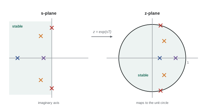
Frequency response follows the same pattern: the discrete frequency response is \( H(e^{j\omega T}) \), the transfer function evaluated around the unit circle. Going once round the circle, from angle 0 to π, covers frequencies from 0 to the Nyquist frequency \( f_s/2 \); going further simply repeats, which is the z-domain view of aliasing.
Worked problem
Mapping a continuous pole
A continuous sensor model has a pole at s = −50 rad/s. Where does it map in the z-plane for sampling at 1 kHz and at 50 Hz? Also map a complex pair at \( -10 \pm 40j \) at 1 kHz.
Show solution
- At 1 kHz (T = 0.001): \( z = e^{-0.05} = 0.951 \).
- At 50 Hz (T = 0.02): \( z = e^{-1} = 0.368 \).
- Complex pair at 1 kHz: radius \( e^{-10 \times 0.001} = 0.990 \), angle \( \pm 40 \times 0.001 = \pm 0.04 \) rad (2.3°).
Answer: Fast sampling puts poles close to z = 1, where small coefficient errors matter: 0.951 versus 0.368. The complex pair sits at radius 0.990 and angle ±2.3°, very near the circle and the real axis. Clustering near z = 1 at high sampling rates is why filters implemented with short fixed-point words can misbehave, and why second-order sections are preferred for high-order filters (lesson 11).
From s to z: discretizing continuous designs
Most filters and controllers are designed in continuous time, then converted to code. The conversion approximates differentiation or integration over one sample. Four methods are common.
- Forward Euler: \( \dot{y} \approx (y[n+1] - y[n])/T \), equivalent to \( s \to (z - 1)/T \). It is the simplest, but it maps part of the stable left half-plane outside the unit circle, so a stable continuous design can become unstable if T is too large relative to its fastest time constant. For a pole at −a it requires \( aT < 2 \).
- Backward Euler: \( \dot{y} \approx (y[n] - y[n-1])/T \), equivalent to \( s \to (z - 1)/(zT) \). It maps the whole left half-plane inside the circle, so it never destabilizes a stable design, but it adds phase lag and damping.
- Tustin (bilinear transform): \( s \to \dfrac{2}{T}\dfrac{z - 1}{z + 1} \), which corresponds to trapezoidal integration. It maps the left half-plane exactly onto the inside of the circle and preserves stability, with better accuracy than either Euler method. It compresses the frequency axis, warping high frequencies, so filters with critical frequencies, such as notches, are designed with frequency prewarping, which makes the discrete response exact at one chosen frequency.
- Zero-order-hold (exact) discretization: computes the discrete system that gives exactly the same samples as the continuous system driven through a zero-order hold, mapping each pole by \( z = e^{sT} \). It is the standard for discretizing plant models for digital control design, and it is what simulation libraries do for state-space models (lesson 12).
| Method | Substitution | Stability preserved? | Typical use |
|---|---|---|---|
| Forward Euler | \( s \to (z - 1)/T \) | No; needs small T | Quick simulation; simple integrators |
| Backward Euler | \( s \to (z - 1)/(zT) \) | Yes | Robust integrators; stiff systems |
| Tustin | \( s \to \frac{2}{T}\frac{z - 1}{z + 1} \) | Yes | Filters and controllers; prewarp for notches |
| Zero-order hold | Poles map by \( z = e^{sT} \) | Yes (exact samples) | Discretizing plants for digital control |
Worked problem
Discretizing a low-pass filter three ways
Convert \( G(s) = \dfrac{a}{s + a} \) with a = 100 rad/s to a difference equation at T = 0.001 s by forward Euler, Tustin and the exact (matched) method.
Show solution
- Forward Euler: \( (z - 1)/T + a \) in the denominator gives \( y[n] = (1 - aT)y[n-1] + aT\,x[n-1] = 0.9\,y[n-1] + 0.1\,x[n-1] \).
- Tustin: \( G = \dfrac{aT(z + 1)}{(2 + aT)z - (2 - aT)} \), so \( y[n] = \tfrac{2 - aT}{2 + aT}y[n-1] + \tfrac{aT}{2 + aT}(x[n] + x[n-1]) = 0.9048\,y[n-1] + 0.0476\,(x[n] + x[n-1]) \).
- Exact (ZOH): pole at \( e^{-aT} = e^{-0.1} = 0.9048 \), giving \( y[n] = 0.9048\,y[n-1] + 0.0952\,x[n-1] \).
Answer: All three are close at this sampling rate because aT = 0.1 is small; Tustin and the exact method even share the same pole, 0.9048, to four figures. Forward Euler's pole of 0.9 is slightly faster. The differences grow quickly as aT increases, as the next example shows.
Worked problem
When forward Euler goes unstable
A stiff current-loop model has a pole at s = −3,000 rad/s. Simulated or implemented with forward Euler at 1 kHz, is it stable? What about Tustin?
Show solution
- Forward Euler maps the pole to \( z = 1 - aT = 1 - 3 = -2 \).
- |z| = 2 > 1: unstable, alternating in sign and doubling every sample.
- Tustin maps it to \( (2 - aT)/(2 + aT) = (2 - 3)/(2 + 3) = -0.2 \), inside the circle: stable.
Answer: Forward Euler turns a perfectly stable fast pole into an exploding oscillation whenever aT > 2; Tustin does not. Simulations of robots with stiff contacts or fast electrical dynamics often blow up for exactly this reason, which is why simulators use implicit or adaptive-step integrators.
import numpy as np
a = 100.0
for T in [0.001, 0.01, 0.025]:
    aT = a*T
    euler = 1 - aT
    tustin = (2 - aT)/(2 + aT)
    exact = np.exp(-aT)
print(f"T = {T*1000:5.1f} ms: pole euler {euler:7.4f} tustin {tustin:7.4f} exact {exact:7.4f}")T = 1.0 ms: pole euler 0.9000 tustin 0.9048 exact 0.9048 T = 10.0 ms: pole euler 0.0000 tustin 0.3333 exact 0.3679 T = 25.0 ms: pole euler -1.5000 tustin -0.1111 exact 0.0821
At 1 ms all three agree; at 10 ms forward Euler places the pole at zero, a filter with no memory at all; at 25 ms it puts the pole at −1.5, outside the unit circle, so the 'filter' is unstable, while Tustin and the exact method stay inside. The lesson for embedded code: either sample fast relative to the dynamics, or use a method that preserves stability.
Common mistakes
MistakeTreating z⁻¹ as a mysterious operator
InsteadIt is simply a one-sample delay: the previous value stored in a variable.
MistakeChecking discrete stability with the left half-plane rule
InsteadDiscrete poles must lie inside the unit circle.
MistakeUsing forward Euler with a sample period near the fastest time constant
InsteadForward Euler needs aT < 2 for stability; use Tustin, backward Euler or exact discretization.
MistakeForgetting frequency warping when discretizing a notch with Tustin
InsteadPrewarp so the notch lands at the intended frequency.
MistakeImplementing a high-order IIR filter as one long difference equation
InsteadSplit it into second-order sections to avoid numerical problems.
Summary and key terms
- Discrete LTI systems are described by difference equations that translate directly into code.
- FIR systems depend only on inputs; IIR systems also feed back past outputs.
- The z-transform turns difference equations into algebra, with z⁻¹ representing a one-sample delay.
- The mapping \( z = e^{sT} \) takes the left half-plane inside the unit circle; discrete systems are stable when all poles are inside it.
- The discrete frequency response is H evaluated on the unit circle, covering 0 to the Nyquist frequency once.
- Forward Euler, backward Euler, Tustin and exact zero-order-hold methods convert continuous designs to discrete ones.
- Forward Euler can destabilize fast poles; Tustin and exact methods preserve stability.
- Difference equation
- An equation relating current and past samples of input and output.
- IIR filter
- A recursive filter whose impulse response continues indefinitely.
- z-transform
- The sum \( \sum x[n]z^{-n} \) that maps a sequence to a function of z.
- Unit delay
- The operation x[n] → x[n − 1], represented by z⁻¹.
- Discrete transfer function
- The ratio Y(z)/X(z) of a discrete LTI system.
- Unit circle
- The set |z| = 1, the discrete stability boundary.
- Forward Euler
- Discretization using s → (z − 1)/T.
- Tustin method
- The bilinear discretization s → (2/T)(z − 1)/(z + 1).
- Frequency prewarping
- Adjusting a Tustin design so it is exact at a chosen frequency.
- Zero-order-hold discretization
- Exact discretization of a system driven by held samples.
Practice problems
Work each problem on paper first, then reveal the answer to check.
Write the transfer function of y[n] = x[n] − x[n − 1].
Show answer
\( 1 - z^{-1} = (z - 1)/z \).
Is y[n] = 1.1 y[n − 1] + x[n] stable?
Show answer
No; its pole at 1.1 is outside the unit circle.
What is the DC gain of \( H(z) = 0.2/(1 - 0.8z^{-1}) \)?
Show answer
H(1) = 0.2/0.2 = 1.
Map a continuous pole at s = −20 rad/s to z at T = 0.01 s.
Show answer
\( e^{-0.2} = 0.819 \).
What behaviour does a discrete pole at z = −0.9 produce?
Show answer
A decaying sequence that alternates sign every sample.
Write the difference equation for \( H(z) = (1 + z^{-1})/(1 - 0.5z^{-1}) \).
Show answer
y[n] = 0.5y[n − 1] + x[n] + x[n − 1].
For forward Euler, what is the largest T that keeps a pole at −400 rad/s stable?
Show answer
T < 2/400 = 5 ms.
Where on the unit circle does the Nyquist frequency lie?
Show answer
At z = −1 (angle π).
Discretize \( 1/s \) with Tustin.
Show answer
\( \frac{T}{2}\frac{z + 1}{z - 1} \), the trapezoidal integrator.
Why do poles cluster near z = 1 at high sampling rates?
Show answer
Because \( e^{-aT} \to 1 \) as T becomes small compared with 1/a.
Lesson quiz · 5 questions
Score 60% or more to complete this lesson.
Create a free account to save your progress, take quizzes and earn a certificate.