
ROB-230 · Lesson 8 of 12 · 30 min
Fourier series, the Fourier transform and the FFT
Lesson 7 showed how an LTI system treats a single sinusoid. Real signals, such as the vibration of a gearbox, the current ripple of a PWM drive or the jitter in an IMU reading, are not single sinusoids, but Joseph Fourier's great insight of 1807 was that they can be built from sinusoids. A periodic signal is a sum of harmonics at multiples of its fundamental frequency; an aperiodic signal is a continuous blend of all frequencies. Knowing which frequencies a signal contains, its spectrum, lets an engineer diagnose a noisy bearing, choose a filter cutoff, pick a sampling rate and predict how a system will respond, by multiplying the input spectrum by the frequency response. And thanks to the fast Fourier transform, an algorithm of 1965 that is among the most important ever devised, computing the spectrum of measured data takes milliseconds. This lesson builds Fourier series and the Fourier transform, connects them to the Laplace transform, and shows how to use the FFT correctly on real robot data.
Fourier series of periodic signals
A periodic signal with period \( T_0 \) and fundamental angular frequency \( \omega_0 = 2\pi/T_0 \) can be written as a sum of harmonics:
The coefficients are found by projecting the signal onto each harmonic, which works because sines and cosines of different harmonics are orthogonal over a period:
The constant \( a_0 \) is the average, or DC, value. The amplitude of the k-th harmonic is \( \sqrt{a_k^2 + b_k^2} \). Using Euler's formula, the series can also be written compactly with complex exponentials, \( x(t) = \sum_k c_k e^{jk\omega_0 t} \), with k running over negative as well as positive integers; negative frequencies are a bookkeeping device that pairs with positive ones to make real signals.
Even signals contain only cosines and odd signals only sines, which halves the work. Sharp edges need many harmonics: the coefficients of a signal with jumps fall off as 1/k, those of a continuous signal with kinked slope as 1/k², and those of smooth signals faster still. This is the mathematical reason fast edges, such as PWM switching or a step command, generate high-frequency content that can excite resonances and cause electromagnetic interference.
Worked problem
Harmonics of a square wave
A PWM signal at 50 % duty cycle switches between −1 and +1 V with period \( T_0 \), an odd square wave. Find its Fourier series.
Show solution
- The wave is odd and has zero average, so \( a_0 = a_k = 0 \).
- \( b_k = \frac{2}{T_0}\left[\int_0^{T_0/2}\sin(k\omega_0t)\,dt - \int_{T_0/2}^{T_0}\sin(k\omega_0t)\,dt\right] = \frac{2}{k\pi}(1 - \cos k\pi) \).
- This is \( 4/(k\pi) \) for odd k and 0 for even k.
- So \( x(t) = \frac{4}{\pi}\left[\sin\omega_0t + \tfrac{1}{3}\sin3\omega_0t + \tfrac{1}{5}\sin5\omega_0t + \cdots\right] \).
Answer: A square wave contains only odd harmonics, with amplitudes 4/π ≈ 1.27, 0.42, 0.25 and so on, falling as 1/k. A motor driven by 20 kHz PWM therefore sees components at 20, 60, 100 kHz and beyond; its inductance filters them, leaving the small current ripple measured in ROB-200.
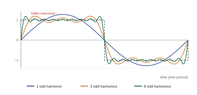
Truncating the series leaves an overshoot of about 9 % of the jump next to each discontinuity, no matter how many terms are kept; this is the Gibbs phenomenon. It reappears whenever a signal is sharply band-limited, for example as ringing near edges when an image or a step is low-pass filtered with a very sharp filter.
Power and Parseval's theorem
Each harmonic carries a share of the signal's power, and the shares add up, because the harmonics are orthogonal. Parseval's theorem states that the average power equals the sum of the powers of the components:
This is the formal version of the rule used in lesson 1 to add RMS values of independent components. For the ±1 V square wave the power is exactly 1 W into 1 Ω; the fundamental alone carries \( (4/\pi)^2/2 = 0.81 \), 81 % of it, and the first three odd harmonics together carry 93 %.
The Fourier transform
Most signals are not periodic: a single impact, a step command, a burst of noise. Letting the period grow without limit squeezes the harmonics together until they form a continuum, and the Fourier series becomes the Fourier transform:
\( X(j\omega) \) is the signal's spectrum: its magnitude says how much of each frequency is present, its phase says how those components line up. Comparing with lesson 5, the Fourier transform is the Laplace transform evaluated on the imaginary axis, for signals where that integral converges. The frequency response \( G(j\omega) \) of lesson 7 is precisely the Fourier transform of the impulse response.
The Fourier transform shares the key properties of the Laplace transform. Convolution in time becomes multiplication in frequency, so an LTI system's output spectrum is \( Y(j\omega) = G(j\omega)X(j\omega) \): the system reshapes the input spectrum by its frequency response. A time delay multiplies the spectrum by \( e^{-j\omega T} \), changing only phase. And there is a fundamental trade-off between duration and bandwidth: a short pulse has a wide spectrum, and a narrow spectrum needs a long signal. A rectangular pulse of width W has a spectrum shaped like \( \sin(\omega W/2)/(\omega W/2) \) whose main lobe is about 1/W hertz wide; the shorter the hammer tap in modal testing, the higher the frequencies it excites.
Worked problem
Spectrum of an impact
An impact hammer used to test a robot arm produces a force pulse lasting about 1 ms. Up to roughly what frequency does it excite the arm usefully? What if a soft rubber tip lengthens the pulse to 5 ms?
Show solution
- A pulse of width W has its first spectral null at f = 1/W.
- 1 ms pulse: null at 1,000 Hz; the spectrum is reasonably flat up to a few hundred hertz.
- 5 ms pulse: null at 200 Hz; useful excitation only up to roughly 100 Hz.
Answer: The hard tip excites modes up to several hundred hertz; the soft tip concentrates energy below about 100 Hz. Test engineers choose the tip to match the frequency range of interest, a direct application of the time-bandwidth trade-off.
From continuous to discrete: the DFT and FFT
Computers handle finite lists of samples, not continuous functions. The discrete Fourier transform (DFT) of N samples \( x[0], \dots, x[N-1] \) taken every T seconds is
Bin k corresponds to frequency \( f_k = k/(NT) = k\,f_s/N \), where \( f_s = 1/T \) is the sampling rate. The spacing between bins, the frequency resolution, is therefore \( \Delta f = f_s/N = 1/(NT) \), the reciprocal of the record length: to resolve two tones 0.5 Hz apart you need at least 2 s of data, whatever the sampling rate. For real signals the spectrum above \( f_s/2 \) mirrors the part below, so only bins 0 to N/2 carry new information; lesson 9 explains why \( f_s/2 \), the Nyquist frequency, is a hard limit.
Computed directly, the DFT needs about N² complex multiplications. The fast Fourier transform (FFT), published by James Cooley and John Tukey in 1965 (building on an idea Gauss had used in 1805), computes exactly the same result in about \( N\log_2 N \) operations by recursively splitting the sum into halves. For N = 1,024 that is about 10,000 operations instead of a million, and for a million samples the speed-up is about 50,000-fold. The FFT is what makes real-time spectrum analysis, fast convolution and modern communications possible.
Worked problem
Choosing FFT parameters for vibration monitoring
You want to detect bearing vibration up to 2 kHz on a robot joint and distinguish components 1 Hz apart. Choose a sampling rate and record length, and find N.
Show solution
- Highest frequency 2 kHz requires \( f_s > 4 \) kHz; with margin for an anti-aliasing filter (lesson 9), choose \( f_s = 10 \) kHz.
- Resolution 1 Hz requires a record of at least \( 1/\Delta f = 1 \) s.
- \( N = f_s \times 1\text{ s} = 10{,}000 \) samples; rounding up to a power of two, 16,384 samples (1.64 s) suits radix-2 FFTs, though modern libraries handle any N efficiently.
Answer: Sample at 10 kHz for at least 1 s, about 10,000 to 16,384 samples, giving 1 Hz or finer resolution up to the 5 kHz Nyquist limit. A longer record improves resolution; a faster sampling rate does not.
Using the FFT on real data: windows and leakage
The DFT implicitly assumes the N samples are one period of a periodic signal. If a sinusoid does not complete a whole number of cycles in the record, the copies do not join smoothly, and the jump spreads the tone's energy into neighbouring bins. This spectral leakage blurs peaks and can hide small components next to large ones. The remedy is a window: multiply the record by a smooth taper, such as the Hann window \( w[n] = 0.5 - 0.5\cos(2\pi n/N) \), that falls to zero at both ends. Windowing trades a slightly wider main peak for much lower leakage. Other practical points: remove the mean (or detrend) first so the DC bin does not swamp the plot; scale magnitudes so a sinusoid of amplitude A shows as A (multiply by 2/N for a rectangular window, and divide also by the window's mean, 0.5 for Hann); and average spectra from several records to reduce the scatter of noise estimates, which is Welch's method.
import numpy as np
fs, Tlen = 1000.0, 2.0                    # 1 kHz for 2 s -> 0.5 Hz bins
N = int(fs*Tlen); t = np.arange(N)/fs
rng = np.random.default_rng(4)
x = 0.8*np.sin(2*np.pi*47.3*t) + 0.05*np.sin(2*np.pi*120*t) + rng.normal(0, 0.1, N)
f = np.fft.rfftfreq(N, 1/fs)
for name, w in [("rectangular", np.ones(N)), ("Hann", np.hanning(N))]:
    X = np.abs(np.fft.rfft((x - x.mean())*w)) * 2/(N*w.mean())
    k47 = np.argmax(X); k120 = np.argmin(np.abs(f - 120))
    near = X[np.argmin(np.abs(f - 55))]
print(f"{name:11s}: peak {X[k47]:.3f} at {f[k47]:.1f} Hz | 120 Hz line {X[k120]:.3f} | floor at 55 Hz {near:.4f}")rectangular: peak 0.604 at 47.5 Hz | 120 Hz line 0.052 | floor at 55 Hz 0.0155 Hann : peak 0.721 at 47.5 Hz | 120 Hz line 0.054 | floor at 55 Hz 0.0063
Both spectra find the 47.3 Hz tone, which falls between the bins at 47.0 and 47.5 Hz, and the small 120 Hz component. With the rectangular window the tone reads only 0.60 instead of its true 0.8, because its energy is split across several bins, and its leakage raises the floor 8 Hz away at 55 Hz. The Hann window reads 0.72, closer to the truth (the remaining shortfall, called scalloping loss, comes from the tone sitting between bins), and its floor near the tone is less than half as high, so small components close to large ones stand out more clearly. In practice, use a window by default, and if accurate amplitudes matter, use a longer record or a flat-top window.
| Quantity | Formula | Controlled by |
|---|---|---|
| Bin spacing (resolution) | \( \Delta f = f_s/N = 1/(NT) \) | Record length |
| Highest frequency in the spectrum | \( f_s/2 \) (Nyquist) | Sampling rate |
| Frequency of bin k | \( k f_s/N \) | Both |
| Amplitude scaling (rectangular) | multiply |X[k]| by 2/N | Window choice |
| FFT cost | about \( N\log_2 N \) operations | Number of samples |
Common mistakes
MistakeExpecting a higher sampling rate to improve frequency resolution
InsteadResolution is 1/(record length); sample for longer to resolve close frequencies.
MistakeReading raw FFT magnitudes as signal amplitudes
InsteadScale by 2/N (and correct for the window) to recover sinusoid amplitudes.
MistakeForgetting to remove the mean before an FFT
InsteadA large DC component dominates the plot and leaks into low bins.
MistakeUsing no window on non-periodic records
InsteadApply a Hann or similar window to suppress leakage.
MistakeInterpreting bins above f_s/2 as real frequencies
InsteadFor real signals they mirror the lower half; only 0 to f_s/2 is meaningful.
Summary and key terms
- A periodic signal is a sum of harmonics at multiples of its fundamental frequency, with coefficients found by projection.
- Sharp edges require many harmonics; a square wave has only odd harmonics falling as 1/k.
- Parseval's theorem says the power of a signal is the sum of the powers of its components.
- The Fourier transform describes aperiodic signals as a continuous spectrum and equals the Laplace transform on the imaginary axis.
- An LTI system multiplies the input spectrum by its frequency response.
- The DFT of N samples has bins spaced f_s/N apart up to the Nyquist frequency f_s/2; the FFT computes it in N log N time.
- Windowing reduces spectral leakage when a record does not contain whole cycles.
- Fourier series
- A representation of a periodic signal as a sum of harmonics.
- Harmonic
- A sinusoid at an integer multiple of the fundamental frequency.
- Spectrum
- The distribution of a signal's content across frequency.
- Fourier transform
- The integral that gives the continuous spectrum of an aperiodic signal.
- Gibbs phenomenon
- The persistent overshoot near discontinuities when a Fourier series is truncated.
- Parseval's theorem
- The equality of a signal's power in time and in frequency.
- DFT
- The discrete Fourier transform of a finite list of samples.
- FFT
- A fast algorithm for computing the DFT in about N log₂ N operations.
- Frequency resolution
- The spacing between DFT bins, equal to the reciprocal of the record length.
- Spectral leakage
- The spreading of a tone into neighbouring bins when the record does not hold whole cycles.
Practice problems
Work each problem on paper first, then reveal the answer to check.
A signal has period 20 ms. What are its first three harmonic frequencies?
Show answer
50, 100 and 150 Hz.
What is the amplitude of the 7th harmonic of a ±1 square wave?
Show answer
\( 4/(7\pi) = 0.182 \).
What fraction of a square wave's power is in its fundamental?
Show answer
About 81 %.
Data are sampled at 2 kHz for 0.5 s. What are the bin spacing and Nyquist frequency?
Show answer
2 Hz and 1 kHz.
How many samples are needed for 0.1 Hz resolution at 500 Hz sampling?
Show answer
5,000 (10 s of data).
Roughly how many operations does a 4,096-point FFT need, compared with a direct DFT?
Show answer
About 49,000 versus about 16.8 million.
A 0.2 ms pulse excites frequencies up to roughly what value?
Show answer
Its first null is at 5 kHz.
An LTI system has gain 0.1 at 60 Hz. A 60 Hz input component of amplitude 3 gives what output amplitude?
Show answer
0.3.
Why does a Hann window reduce leakage?
Show answer
It tapers the record to zero at both ends, removing the jump between repeated copies.
A DFT bin at k = 250 with N = 4,000 and f_s = 8 kHz corresponds to which frequency?
Show answer
500 Hz.
Lesson quiz · 5 questions
Score 60% or more to complete this lesson.
Create a free account to save your progress, take quizzes and earn a certificate.