
ROB-230 · Lesson 9 of 12 · 34 min
Sampling, aliasing and reconstruction
Every robot controller is a computer, and computers see the continuous world only through samples. An ADC reads a current sensor 20,000 times a second, an IMU delivers 1,000 readings a second, a joint controller updates its command every millisecond. Between samples the computer is blind, and after computing a command it holds that value until the next update. Both steps change the signals in ways that matter. Sample too slowly and high frequencies masquerade as low ones, an effect called aliasing that can make a vibrating machine appear to drift or turn a 50 Hz electrical hum into a slow wobble that no later filter can remove. Hold commands for too long and the loop acquires extra delay that erodes stability. This lesson explains the sampling theorem, aliasing and how to prevent it with anti-aliasing filters, quantization noise, and the zero-order hold that turns samples back into continuous signals.
Ideal sampling
Sampling a continuous signal x(t) every T seconds produces the sequence \( x[n] = x(nT) \). The sampling rate is \( f_s = 1/T \) samples per second (hertz), or \( \omega_s = 2\pi/T \) in radians per second. A useful mental model writes the sampled signal as the continuous signal multiplied by a train of impulses spaced T apart. In the frequency domain, multiplication becomes convolution, and the spectrum of an impulse train is another impulse train, spaced \( f_s \) apart. The result is the single most important fact about sampling: the spectrum of a sampled signal is the original spectrum repeated, or replicated, at every multiple of the sampling rate:
If the original spectrum is confined to frequencies below \( f_s/2 \), the copies do not overlap and the original can be recovered exactly. If it extends beyond \( f_s/2 \), the copies overlap and the information is scrambled irreversibly.
The sampling theorem
The Nyquist-Shannon sampling theorem, developed by Harry Nyquist (1928), Claude Shannon (1949) and earlier by Vladimir Kotelnikov (1933), states: a signal containing no frequencies at or above B hertz is completely determined by samples taken at a rate \( f_s > 2B \). The frequency \( f_s/2 \) is called the Nyquist frequency, and 2B the Nyquist rate. Below the Nyquist frequency, sampling loses nothing. In practice, engineers sample several times faster than 2B, for three reasons: real anti-aliasing filters do not cut off sharply, control loops need many samples per response time to keep the delay of sampling small, and reconstruction with a simple hold is crude unless samples are close together. Common rules of thumb are 5 to 10 times the highest frequency of interest for measurement and 10 to 30 times the closed-loop bandwidth for digital control.
Aliasing
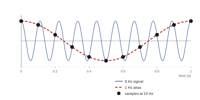
What happens to a frequency above the Nyquist frequency? It appears, after sampling, at a lower alias frequency. A sinusoid at frequency f produces exactly the same samples as one at \( |f - kf_s| \) for any integer k, and the observed frequency is the one that falls between 0 and \( f_s/2 \):
The figure shows the classic case: a 9 Hz sinusoid sampled at 10 Hz yields samples indistinguishable from a 1 Hz sinusoid. The same effect makes wagon wheels in films appear to turn slowly backwards, and makes a spinning propeller filmed with a rolling-shutter camera look bent. In a robot, aliasing can turn high-frequency vibration, PWM ripple or electrical hum into apparent slow motion that the controller then tries to correct, causing real low-frequency movement. Once aliased, the false component lies in the same band as the true signal and no digital filter can separate them. Aliasing must be prevented before sampling.
Worked problem
Finding an alias
A joint's current sensor picks up a 950 Hz vibration-induced component. The current is sampled at 1 kHz for a slow torque estimate. At what frequency does the component appear? What if the sampling rate is 1.2 kHz?
Show solution
- At \( f_s = 1000 \) Hz, Nyquist is 500 Hz. \( |950 - 1 \times 1000| = 50 \) Hz.
- At \( f_s = 1200 \) Hz, Nyquist is 600 Hz. \( |950 - 1 \times 1200| = 250 \) Hz.
Answer: At 1 kHz the vibration masquerades as a 50 Hz oscillation, right where the torque loop operates, and could be mistaken for a real load change. At 1.2 kHz it appears at 250 Hz, easier to filter digitally but still false. The real fix is an analogue anti-aliasing filter that removes the 950 Hz component before the ADC.
Worked problem
Mains hum and a slow sample rate
A strain-gauge amplifier picks up 60 Hz mains interference and is read by a microcontroller at 59 Hz. What appears in the data?
Show solution
- Nyquist is 29.5 Hz, so 60 Hz aliases.
- \( |60 - 1 \times 59| = 1 \) Hz.
Answer: The hum appears as a slow 1 Hz oscillation that looks exactly like a real load fluctuation. Sampling at a rate that is an exact multiple of the mains frequency, or integrating over whole mains cycles, as many precision ADCs do, makes the interference average to zero instead; in regions with 50 Hz mains the same idea applies at multiples of 50 Hz.
Anti-aliasing filters
The defence against aliasing is an analogue low-pass filter in front of the ADC that removes content above the Nyquist frequency, or at least attenuates it below the resolution of the converter. Because no real filter has a vertical cutoff, the filter's passband edge must sit well below \( f_s/2 \), and the gap between them, the transition band, determines how steep, and therefore how complex, the filter must be. A first-order RC filter rolls off at only 20 dB per decade; reaching the 72 dB that matches a 12-bit ADC's resolution would take more than three decades of margin. Higher-order active filters (Butterworth, Bessel) roll off at 20n dB per decade for order n. The modern alternative is oversampling: sample an inexpensive sigma-delta ADC at a very high rate, where a simple RC filter suffices, then filter and decimate digitally to the rate actually needed. Most MEMS IMUs and audio converters work this way, with configurable digital low-pass filters, which is why IMU datasheets list an output data rate and a separate bandwidth setting (ROB-220).
Worked problem
Sizing an anti-aliasing filter
A force sensor signal of interest extends to 50 Hz and is sampled at 1 kHz with a 12-bit ADC. Interference above 500 Hz must be attenuated by at least 60 dB. What order of Butterworth filter with a 100 Hz cutoff is needed?
Show solution
- An n-th order Butterworth filter attenuates by about 20n dB per decade above its cutoff.
- From 100 Hz to 500 Hz is \( \log_{10}5 = 0.70 \) decades.
- Required: \( 20n \times 0.70 \ge 60 \), so \( n \ge 4.3 \); choose n = 5.
- Check the passband: at 50 Hz a fifth-order Butterworth with 100 Hz cutoff has gain \( 1/\sqrt{1 + 0.5^{10}} = 0.9995 \), essentially flat.
Answer: A fifth-order Butterworth filter at 100 Hz meets the requirement. Alternatively, sampling at 5 kHz and decimating digitally would let a much simpler analogue filter do the job, which is why oversampling has largely replaced steep analogue filters.
Quantization
Sampling discretizes time; quantization discretizes amplitude. An N-bit ADC with full-scale range V resolves steps of \( \Delta = V/2^N \) (ROB-200). The rounding error is at most \( \Delta/2 \) and, for busy signals, behaves like uniform random noise with standard deviation
The resulting signal-to-quantization-noise ratio for a full-scale sinusoid is about \( 6.02N + 1.76 \) dB: 74 dB for 12 bits, 98 dB for 16 bits. Each extra bit buys 6 dB. Oversampling also helps here: averaging four samples halves the noise, which is worth one extra bit, so oversampling by \( 4^k \) gains k bits, provided the noise is genuinely random. Quantization in encoders works the same way: an encoder of resolution q radians adds noise of \( q/\sqrt{12} \) to every angle reading, which matters when angles are differenced to get velocity (lesson 11).
Worked problem
Quantization noise of an encoder
A joint encoder has 4,096 counts per revolution. Find the quantization step, the RMS quantization noise, and the RMS noise of a velocity estimate formed by differencing consecutive readings at 1 kHz.
Show solution
- Step \( q = 2\pi/4096 = 1.534 \times 10^{-3} \) rad.
- RMS noise \( q/\sqrt{12} = 4.43 \times 10^{-4} \) rad.
- A difference of two independent errors has RMS \( \sqrt{2} \times 4.43 \times 10^{-4} = 6.27 \times 10^{-4} \) rad; dividing by T = 0.001 s gives 0.627 rad/s.
Answer: Position noise is a tiny 0.44 mrad, but the differenced velocity has about 0.63 rad/s (36 °/s) of noise at 1 kHz, larger than many slow motions. Faster sampling makes differencing worse, not better, which is why velocity is usually estimated by filtering, period measurement or an observer.
Reconstruction and the zero-order hold
Going the other way, a controller's discrete commands must become a continuous voltage or current. The ideal reconstruction implied by the sampling theorem uses a perfect low-pass filter, which would need an infinite, non-causal impulse response, impossible in real time. Instead, digital-to-analogue converters and PWM stages use a zero-order hold (ZOH): each command is held constant until the next one arrives, producing a staircase. The ZOH has impulse response equal to a rectangle of width T, and its transfer function is
Its frequency response has a magnitude shaped like \( \sin(\omega T/2)/(\omega T/2) \) and, most importantly, a phase lag of \( \omega T/2 \): on average the staircase lags the smooth signal by half a sample. In a control loop this is an effective delay of T/2 on top of computation and sensor delays. At a loop crossover frequency \( \omega_c \), the lost phase margin is \( \omega_c T/2 \) radians. This is the quantitative reason digital controllers must sample well above their bandwidth.
Worked problem
Phase lost to sampling
A joint position loop has a gain crossover of 30 Hz. How much phase margin does the zero-order hold cost at sampling rates of 200 Hz, 1 kHz and 10 kHz, counting also one full sample of computation delay?
Show solution
- Total effective delay \( T/2 + T = 1.5T \); phase lost \( = 360° \times f_c \times 1.5T \).
- 200 Hz (T = 5 ms): \( 360 \times 30 \times 0.0075 = 81° \).
- 1 kHz (T = 1 ms): \( 360 \times 30 \times 0.0015 = 16.2° \).
- 10 kHz: \( 1.6° \).
Answer: At 200 Hz sampling the delays consume 81°, more than any reasonable phase margin, so the loop would be unstable; at 1 kHz they cost 16°, significant but manageable; at 10 kHz they are negligible. This is why servo drives run current loops at 10 to 40 kHz and position loops at 1 to 8 kHz.
import numpy as np
fs = 1000.0
for f in [50, 450, 550, 950, 1050, 1950]:
    n = np.arange(2000)
    x = np.cos(2*np.pi*f*n/fs)                      # sampled cosine
    X = np.abs(np.fft.rfft(x*np.hanning(n.size)))
    f_obs = np.fft.rfftfreq(n.size, 1/fs)[np.argmax(X)]
    k = round(f/fs); f_pred = abs(f - k*fs)
print(f"true {f:5.0f} Hz -> observed {f_obs:6.1f} Hz (predicted alias {f_pred:5.0f} Hz)")true 50 Hz -> observed 50.0 Hz (predicted alias 50 Hz) true 450 Hz -> observed 450.0 Hz (predicted alias 450 Hz) true 550 Hz -> observed 450.0 Hz (predicted alias 450 Hz) true 950 Hz -> observed 50.0 Hz (predicted alias 50 Hz) true 1050 Hz -> observed 50.0 Hz (predicted alias 50 Hz) true 1950 Hz -> observed 50.0 Hz (predicted alias 50 Hz)
Frequencies below 500 Hz appear where they should; every frequency above it folds back into the 0 to 500 Hz band exactly as the alias formula predicts. A 950 Hz and a 1,050 Hz component both land at 50 Hz, indistinguishable from a genuine 50 Hz signal.
| Design choice | Rule of thumb | Reason |
|---|---|---|
| Measurement sampling rate | 5 to 10 × highest frequency of interest | Room for a practical anti-aliasing filter |
| Digital control loop rate | 10 to 30 × closed-loop bandwidth | Keep sample-and-hold phase lag small |
| Anti-aliasing filter | Attenuate content above f_s/2 below ADC resolution | Aliased content cannot be removed later |
| Oversampling | Sample fast, filter and decimate digitally | Simpler analogue filter; extra effective bits |
| Mains interference | Sample at multiples of 50 or 60 Hz or integrate whole cycles | Hum averages to zero |
Common mistakes
MistakeSampling at exactly twice the highest frequency
InsteadThe theorem requires more than 2B, and practical filters need a wide margin; sample several times faster.
MistakeTrying to remove aliasing with a digital filter after the ADC
InsteadAliased components overlap the true band; filter in analogue before sampling.
MistakeAssuming faster sampling always improves differenced velocity
InsteadQuantization noise in a difference grows as the sample period shrinks.
MistakeIgnoring the half-sample delay of the zero-order hold
InsteadInclude T/2 plus computation delay when checking phase margin.
MistakeChoosing an IMU output rate without checking its bandwidth setting
InsteadConfigure the internal digital low-pass filter to suit the output data rate.
Summary and key terms
- Sampling replicates a signal's spectrum at every multiple of the sampling rate.
- The sampling theorem says a signal with no content at or above B is captured fully by sampling faster than 2B.
- Frequencies above the Nyquist frequency fold back to alias frequencies that cannot be removed afterwards.
- Analogue anti-aliasing filters, or oversampling with digital decimation, must remove high frequencies before sampling.
- Quantization adds noise of standard deviation Δ/√12; each extra bit gains about 6 dB.
- The zero-order hold reconstructs a staircase and adds an effective delay of half a sample.
- Digital control loops should sample 10 to 30 times faster than their bandwidth.
- Sampling rate
- The number of samples taken per second, f_s = 1/T.
- Nyquist frequency
- Half the sampling rate, the highest frequency that can be represented.
- Sampling theorem
- The result that a band-limited signal is fully determined by samples taken faster than twice its bandwidth.
- Aliasing
- The appearance of a high frequency as a false lower frequency after sampling.
- Alias frequency
- The apparent frequency |f − k f_s| in the band 0 to f_s/2.
- Anti-aliasing filter
- An analogue low-pass filter placed before an ADC.
- Oversampling
- Sampling much faster than needed, then filtering and decimating digitally.
- Quantization noise
- The rounding error of an ADC, modelled as noise of standard deviation Δ/√12.
- Zero-order hold
- A reconstruction that holds each sample constant until the next.
- Decimation
- Reducing the sample rate after digital low-pass filtering.
Practice problems
Work each problem on paper first, then reveal the answer to check.
What is the Nyquist frequency for a 400 Hz sampling rate?
Show answer
200 Hz.
A 130 Hz signal is sampled at 100 Hz. Where does it appear?
Show answer
30 Hz.
A 260 Hz signal is sampled at 100 Hz. Where does it appear?
Show answer
|260 − 300| = 40 Hz.
What minimum sampling rate captures a signal band-limited to 3 kHz?
Show answer
More than 6 kHz.
What is the RMS quantization noise of a 10-bit ADC with a 5 V range?
Show answer
\( (5/1024)/\sqrt{12} = 1.41 \) mV.
What is the theoretical SNR of a 14-bit ADC for a full-scale sine?
Show answer
About 86 dB.
How much oversampling gains two extra bits?
Show answer
16 times.
What phase lag does a ZOH at 2 kHz sampling add at 100 Hz?
Show answer
\( 360 \times 100 \times 0.00025 = 9° \).
A control loop has 5 Hz bandwidth. What sampling rate range is sensible?
Show answer
50 to 150 Hz, more for comfort.
Why can't a digital filter remove an alias?
Show answer
After sampling, the alias occupies the same frequency band as the genuine signal.
Lesson quiz · 5 questions
Score 60% or more to complete this lesson.
Create a free account to save your progress, take quizzes and earn a certificate.