
ROB-230 · Lesson 4 of 12 · 28 min
Differential equations and first- and second-order responses
Convolution tells us how to compute an LTI system's output once we know its impulse response, but where do impulse responses come from? For physical systems, the answer is physics: Newton's laws, Kirchhoff's laws and the motor equations of ROB-220 produce linear ordinary differential equations, and solving them gives the impulse and step responses. This lesson models three components found in every robot, an RC filter, a mass-spring-damper and a DC motor, and shows that their behaviour falls into two families. First-order systems respond with a single exponential characterized by a time constant. Second-order systems can overshoot and oscillate, characterized by a natural frequency and a damping ratio. These few parameters, and the specifications built on them such as rise time, overshoot and settling time, are the everyday language in which robot engineers describe and tune their machines.
From physics to differential equations
An RC low-pass filter, the anti-aliasing filter in front of an ADC (ROB-200), has a resistor R in series and a capacitor C to ground. The capacitor current is \( C\,\dot{v}_{\text{out}} \) and equals the resistor current \( (v_{\text{in}} - v_{\text{out}})/R \), so
A mass m on a spring of stiffness k with viscous damping b, pushed by a force F, obeys Newton's second law, \( m\ddot{x} = F - kx - b\dot{x} \), or
This one equation models a surprising range of robot behaviour: a joint under a proportional-derivative controller (where the controller supplies the spring and damper), the flexible coupling of a series elastic actuator (ROB-220), the bounce of a legged robot's foot, and the wobble of a camera on a mast.
A DC motor (ROB-220) with armature resistance R, inductance L, torque constant \( k_t \), back-EMF constant \( k_e \), rotor inertia J and viscous friction b obeys an electrical and a mechanical equation:
The two equations are coupled through the current and the speed. When the electrical time constant L/R is much shorter than the mechanical one, as it usually is, the inductance can be neglected, \( i = (v - k_e\omega)/R \), and the motor reduces to a single first-order equation for speed:
Back-EMF acts like extra damping, \( k_t k_e/R \), which is usually much larger than mechanical friction. This electrical damping is why a DC motor settles to a steady speed for a given voltage.
First-order systems
Every first-order LTI system can be written in the standard form
with time constant \( \tau \) and steady-state gain K. For the RC filter, \( \tau = RC \) and K = 1; for the simplified motor, \( \tau = J/(b + k_tk_e/R) \) and \( K = (k_t/R)/(b + k_tk_e/R) \). The response to a step of height A from rest is
The time constant has a memorable meaning: after one \( \tau \) the output has covered 63.2 % of its final change, after 2\( \tau \) 86.5 %, after 3\( \tau \) 95.0 % and after 4\( \tau \) 98.2 %. The initial slope is \( KA/\tau \): if the output kept rising at its initial rate it would arrive in exactly one time constant. The 10 to 90 % rise time is \( 2.2\tau \), and the 2 % settling time is about \( 4\tau \). A first-order system never overshoots. Its impulse response is \( (K/\tau)\,e^{-t/\tau} \), as lesson 3 used for the temperature sensor.
Worked problem
Time constant of a DC motor
A motor has \( k_t = k_e = 0.05 \) N·m/A (V·s/rad), R = 1.0 Ω, rotor plus load inertia \( J = 2 \times 10^{-4} \) kg·m² and negligible friction. Find the mechanical time constant and the no-load speed and time to 95 % of it after a 12 V step.
Show solution
- Effective damping \( k_tk_e/R = 0.0025 \) N·m·s/rad.
- \( \tau = J/(k_tk_e/R) = 2 \times 10^{-4}/0.0025 = 0.08 \) s.
- Gain \( K = (k_t/R)/(k_tk_e/R) = 1/k_e = 20 \) rad/s per volt, so final speed \( 12 \times 20 = 240 \) rad/s (2,290 rpm).
- 95 % is reached at \( 3\tau = 0.24 \) s.
Answer: The motor behaves as a first-order system with τ = 80 ms, reaching about 228 rad/s, 95 % of 240 rad/s, in 0.24 s. Doubling the load inertia doubles τ, so a heavier arm responds proportionally more slowly.
Second-order systems
The mass-spring-damper is the prototype second-order system. Dividing by m and introducing two new parameters puts it in standard form:
The undamped natural frequency \( \omega_n \) is the frequency at which the system would oscillate with no damping. The damping ratio \( \zeta \) (zeta) is the ratio of the actual damping to the critical damping \( 2\sqrt{km} \), the smallest damping that prevents oscillation. The damping ratio divides second-order behaviour into regimes:
- Underdamped, \( 0 < \zeta < 1 \): the response overshoots and oscillates with a decaying envelope at the damped frequency \( \omega_d = \omega_n\sqrt{1 - \zeta^2} \).
- Critically damped, \( \zeta = 1 \): the fastest response without overshoot.
- Overdamped, \( \zeta > 1 \): sluggish, no overshoot, behaving like two first-order systems in series.
- Undamped, \( \zeta = 0 \): oscillation forever at \( \omega_n \). Negative damping means instability.
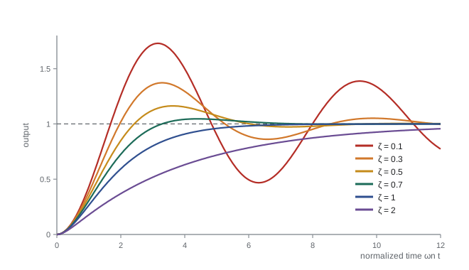
For an underdamped system, the step response from rest is
Its shape is summarized by a few specifications that appear on every control datasheet and in every tuning discussion:
| Specification | Formula (underdamped) | Meaning |
|---|---|---|
| Percent overshoot | \( 100\,e^{-\pi\zeta/\sqrt{1-\zeta^2}} \) | How far the peak exceeds the final value |
| Peak time | \( \pi/\omega_d \) | Time to the first peak |
| Rise time (10 to 90 %) | roughly \( 1.8/\omega_n \) for ζ near 0.5; longer for heavier damping | Speed of the initial response |
| 2 % settling time | about \( 4/(\zeta\omega_n) \) | Time to stay within 2 % of final value |
| Damped frequency | \( \omega_n\sqrt{1 - \zeta^2} \) | Frequency of the visible ringing |
Overshoot depends only on \( \zeta \): 73 % at \( \zeta = 0.1 \), 37 % at 0.3, 16 % at 0.5, 4.6 % at 0.7 and none at 1. A damping ratio around 0.7 is a popular compromise, fast with little overshoot. Settling time depends on \( \zeta\omega_n \), the rate at which the envelope decays. Raising stiffness raises \( \omega_n \) and speeds everything up; adding damping reduces overshoot but, past critical damping, slows the response.
Worked problem
A joint under PD control
A joint with inertia 0.02 kg·m² is controlled by a PD law with stiffness \( K_p = 8 \) N·m/rad and damping \( K_d = 0.4 \) N·m·s/rad. Find \( \omega_n \), \( \zeta \), overshoot, peak time and settling time for a step command.
Show solution
- \( \omega_n = \sqrt{8/0.02} = 20 \) rad/s.
- \( \zeta = 0.4/(2\sqrt{8 \times 0.02}) = 0.4/0.8 = 0.5 \).
- Overshoot \( = 100\,e^{-\pi \times 0.5/0.866} = 16.3 \) %.
- \( \omega_d = 20 \times 0.866 = 17.3 \) rad/s, peak time \( \pi/17.3 = 0.181 \) s; settling time \( 4/(0.5 \times 20) = 0.4 \) s.
Answer: The joint overshoots by 16 %, peaks at 0.18 s and settles within 2 % in about 0.4 s. To cut the overshoot to about 5 % without changing the speed, raise \( K_d \) to give ζ = 0.7: \( K_d = 2 \times 0.7 \times \sqrt{8 \times 0.02} = 0.56 \).
Worked problem
Identifying a system from its step response
A camera gimbal axis, given a small step command, overshoots by 25 % and its oscillation has a period of 0.5 s. Estimate \( \zeta \) and \( \omega_n \).
Show solution
- Invert the overshoot formula: \( \zeta = -\ln(0.25)/\sqrt{\pi^2 + \ln^2 0.25} = 1.386/\sqrt{9.870 + 1.922} = 1.386/3.434 = 0.404 \).
- \( \omega_d = 2\pi/0.5 = 12.57 \) rad/s.
- \( \omega_n = \omega_d/\sqrt{1 - \zeta^2} = 12.57/0.915 = 13.7 \) rad/s.
Answer: About ζ = 0.40 and \( \omega_n \) = 13.7 rad/s (2.2 Hz). Reading these two numbers off a single step test is one of the quickest ways to characterize a mechanism before tuning its controller.
Natural response, forced response and the characteristic equation
Why exponentials? Try \( y = e^{st} \) in the homogeneous equation (input zero). Every derivative brings down a factor s, so \( s^2 + 2\zeta\omega_n s + \omega_n^2 = 0 \), the characteristic equation. Its roots
determine the natural response. Real, negative roots give decaying exponentials (overdamped); a repeated root gives critical damping; complex roots \( -\zeta\omega_n \pm j\omega_d \) give decaying oscillation; roots with positive real part give growth, which is instability. The total response is the natural response, set by initial conditions, plus a forced response that has the same form as the input: a constant for a step, a sinusoid at the input frequency for a sinusoidal input. These roots reappear in lesson 5 as the poles of the transfer function, and their location in the complex plane becomes the main way of thinking about system behaviour.
Simulating responses numerically
Analytical solutions exist for first- and second-order systems, but real robot models quickly get more complicated, so numerical simulation is essential. The simplest method, forward Euler, replaces derivatives by differences over a small step h: \( y_{k+1} = y_k + h\,\dot{y}_k \). The step must be well below the fastest time constant, or the simulation becomes inaccurate or even unstable (lesson 10 explains why). The code below simulates the PD-controlled joint from the example and measures its overshoot and settling time directly.
import numpy as np
J, Kp, Kd = 0.02, 8.0, 0.4
h, T = 1e-4, 1.0
n = int(T/h)
th, w = 0.0, 0.0
traj = np.empty(n)
for k in range(n):
    tau = Kp*(1.0 - th) - Kd*w        # PD torque for a unit step command
    w += h * tau / J
    th += h * w
    traj[k] = th
t = np.arange(n)*h
over = (traj.max() - 1.0)*100
outside = np.where(np.abs(traj - 1.0) > 0.02)[0]
print(f"overshoot      = {over:.1f} %  (formula 16.3 %)")
print(f"peak time      = {t[traj.argmax()]:.3f} s  (formula 0.181 s)")
print(f"2% settling = {t[outside[-1]]:.3f} s (rule of thumb 0.4 s)")overshoot = 16.3 % (formula 16.3 %) peak time = 0.181 s (formula 0.181 s) 2% settling = 0.403 s (rule of thumb 0.4 s)
The simulated overshoot and peak time match the formulas closely. The measured settling time also lands close to the 4/(ζω_n) rule of thumb, although that rule is only approximate: it follows the decay envelope rather than the actual curve, so for other damping ratios it can be off by 10 to 20 %.
Common mistakes
MistakeReading the time constant as the time to reach the final value
InsteadOne time constant reaches 63.2 %; allow about 4τ to settle within 2 %.
MistakeConfusing the natural frequency with the damped frequency
InsteadThe visible ringing is at \( \omega_d = \omega_n\sqrt{1 - \zeta^2} \), slightly below \( \omega_n \).
MistakeAssuming more damping always gives a faster response
InsteadBeyond critical damping the response becomes slower.
MistakeIgnoring back-EMF when modelling a motor
InsteadBack-EMF adds damping \( k_tk_e/R \), usually larger than friction.
MistakeUsing an Euler step comparable to the system time constant
InsteadKeep the step at least ten times smaller than the fastest time constant.
Summary and key terms
- Physical laws give linear differential equations for RC filters, mass-spring-dampers and DC motors.
- First-order systems are described by a time constant and a gain and respond with a single exponential.
- After one time constant a first-order step response reaches 63.2 %, after four about 98 %.
- Second-order systems are described by a natural frequency and a damping ratio.
- The damping ratio sets overshoot; the product ζω_n sets settling time.
- Roots of the characteristic equation determine the natural response and stability.
- Numerical simulation with a small enough step reproduces the analytical responses and handles more complex models.
- Time constant
- The time for a first-order system to cover 63.2 % of a step change.
- Steady-state gain
- The ratio of final output change to input change.
- Natural frequency
- The frequency at which a second-order system would oscillate with no damping.
- Damping ratio
- Actual damping divided by critical damping.
- Critical damping
- The smallest damping that prevents overshoot.
- Overshoot
- The amount by which the peak exceeds the final value, usually in percent.
- Settling time
- The time after which the response stays within a band, often 2 %, of the final value.
- Rise time
- The time to rise from 10 % to 90 % of the final value.
- Characteristic equation
- The polynomial equation whose roots give the exponents of the natural response.
- Back-EMF
- The voltage generated by a spinning motor, proportional to speed.
Practice problems
Work each problem on paper first, then reveal the answer to check.
An RC filter has R = 10 kΩ and C = 1 µF. What is its time constant?
Show answer
10 ms.
A first-order system with τ = 0.5 s receives a step. When does it reach 95 %?
Show answer
At 1.5 s (3τ).
A mass of 2 kg on a 200 N/m spring has what natural frequency?
Show answer
10 rad/s (1.59 Hz).
What damping b gives critical damping for that mass and spring?
Show answer
\( 2\sqrt{200 \times 2} = 40 \) N·s/m.
Find the overshoot for ζ = 0.7.
Show answer
About 4.6 %.
A system has ζ = 0.2 and \( \omega_n \) = 50 rad/s. Estimate its 2 % settling time.
Show answer
\( 4/(0.2 \times 50) = 0.4 \) s.
Find the roots of \( s^2 + 4s + 13 = 0 \) and describe the response.
Show answer
\( -2 \pm 3j \): decaying oscillation at 3 rad/s.
A motor has \( k_e = 0.1 \) V·s/rad. What is its no-load speed at 24 V, ignoring friction?
Show answer
240 rad/s.
Doubling stiffness k multiplies \( \omega_n \) by what factor?
Show answer
\( \sqrt{2} \approx 1.41 \).
Why does the overdamped response behave like two first-order systems?
Show answer
Its two real roots each give a decaying exponential with its own time constant.
Lesson quiz · 5 questions
Score 60% or more to complete this lesson.
Create a free account to save your progress, take quizzes and earn a certificate.