Robust, adaptive and digital control in practice

The controllers of the previous lessons were designed for a model, and they were analysed in continuous time. Real robots differ from their models: payloads change, friction drifts with temperature and wear, gearboxes flex and cables pull. Real controllers run on computers with finite sample rates, delays, jitter and quantized signals, and drive actuators with hard limits. This lesson gathers the practical knowledge that bridges theory and a working robot: how to make controllers robust to model error, how to let them adapt to unknown parameters, how to estimate parameters from data, how to structure motion control as cascaded current, velocity and position loops, and how to implement everything in discrete time without losing the properties designed in continuous time.

Sources of uncertainty

Model error in robots comes from a handful of predictable sources. Payload is the largest variable one: a robot rated for 10 kg may carry anything from nothing to 10 kg, and the payload's inertia and centre of mass change with how it is gripped. Friction varies with temperature (cold grease can double it), speed, load and wear. Link and gearbox stiffness are known only approximately, and cables and hoses add forces that are hard to model. Inertial parameters from CAD omit fasteners, wiring and paint. Finally, unmodelled dynamics, such as motor inductance, sensor filters, delays and structural modes, are deliberately left out of control models but limit the achievable bandwidth. Robust control accepts the uncertainty and designs for its worst case; adaptive control reduces it by learning; identification reduces it in advance.

Robustness through high gain and integral action

The simplest robustness comes from feedback itself. Model error enters computed torque control as a disturbance η (lesson 9), and the error it causes falls in proportion to the feedback gains. Integral action removes the steady part completely. The limit is set by the unmodelled dynamics: gains high enough to suppress large model errors push the loop bandwidth toward resonances and delays, which the stability margins of lesson 5 forbid. A rule of thumb is that feedback can tolerate model errors whose effect is well below the disturbance-rejection capability at the chosen bandwidth, and anything larger needs better modelling or adaptation.

Sliding mode and robust control

Sliding mode control makes robustness explicit. Define a sliding variable that combines error and its rate, \( s = \dot{e} + \lambda e \); if s is kept at zero, the error decays as \( e^{-\lambda t} \) regardless of the dynamics. The controller adds a switching term large enough to dominate the worst-case uncertainty:

where \( |\eta|_{\max} \) bounds the model-error acceleration and sat is a saturation function that replaces the ideal discontinuous sign function inside a thin boundary layer of width φ. The pure sign function would guarantee perfect tracking but cause chattering, rapid switching that excites resonances and wears actuators; the boundary layer trades a small residual error, of order \( \phi/\lambda \), for smooth control. Sliding mode is used where uncertainty bounds are known and robustness matters more than smoothness, for example in some legged robots and underwater vehicles. Other robust methods, such as \( H_\infty \) design, shape the closed loop to tolerate uncertainty described in the frequency domain.

The disturbance observer

A practical robust technique popular in industrial servo drives is the disturbance observer (DOB). It compares the torque commanded with the torque implied by the measured acceleration and a nominal inertia, and treats the difference as an estimated disturbance:

where Q(s) is a low-pass filter. Subtracting \( \hat{d} \) from the next torque command cancels friction, gravity errors, payload changes and coupling within the filter bandwidth, making the joint behave like the nominal inertia \( \hat{J} \). The outer controller can then be designed for the nominal model. The filter bandwidth sets the trade-off: wider rejects more disturbance but amplifies acceleration noise and erodes stability margins. A DOB essentially gives integral-like disturbance rejection without the overshoot penalty of a large integrator.

Adaptive control and parameter identification

Adaptive control estimates uncertain parameters while the robot runs and uses the estimates in a model-based controller. It relies on the linear-in-parameters property of lesson 2: \( \mathbf{M}\ddot{\mathbf{q}} + \mathbf{C}\dot{\mathbf{q}} + \mathbf{g} = \mathbf{Y}(\mathbf{q},\dot{\mathbf{q}},\ddot{\mathbf{q}})\boldsymbol{\theta} \). The Slotine–Li adaptive controller, from 1987, combines a computed-torque-like law using the current estimate \( \hat{\boldsymbol{\theta}} \) with an update law \( \dot{\hat{\boldsymbol{\theta}}} = -\boldsymbol{\Gamma}\mathbf{Y}^{\mathsf{T}}\mathbf{s} \), driven by a sliding-like error s and an adaptation gain Γ. A Lyapunov proof, again using the skew-symmetry of \( \dot{\mathbf{M}} - 2\mathbf{C} \), shows that tracking errors converge to zero. Parameter estimates converge to the true values only if the trajectory is persistently exciting, that is, rich enough in motion to reveal every parameter.

Offline identification uses the same structure without real-time adaptation. The robot follows an exciting trajectory, joint torques (from motor currents) and motions are recorded, and the parameter vector is found by least squares, stacking the regressor for every sample: \( \hat{\boldsymbol{\theta}} = (\mathbf{Y}^{\mathsf{T}}\mathbf{Y})^{-1}\mathbf{Y}^{\mathsf{T}}\boldsymbol{\tau} \). Payload identification, a common feature of industrial robots, runs a short test motion after the robot picks up a tool and estimates its mass and centre of mass the same way.

import numpy as np
rng = np.random.default_rng(3)
# true single-link parameters: inertia, gravity coefficient m*g*lc, viscous, Coulomb friction
theta_true = np.array([0.43, 10.24, 0.8, 1.5])
t = np.linspace(0, 6, 3001)
q = 0.6*np.sin(1.3*t) + 0.3*np.sin(3.1*t + 0.5)      # exciting trajectory
qd = np.gradient(q, t); qdd = np.gradient(qd, t)
Y = np.column_stack([qdd, np.cos(q), qd, np.sign(qd)])   # regressor
tau = Y @ theta_true + rng.normal(0, 0.15, t.size)       # measured torque with noise
theta_hat, *_ = np.linalg.lstsq(Y, tau, rcond=None)
for name, tr, est in zip(["I", "m g lc", "b", "Fc"], theta_true, theta_hat):
    print(f"{name:7s} true {tr:6.3f}  estimated {est:6.3f}")
print(f"condition number of Y: {np.linalg.cond(Y):.1f}")

I       true  0.430  estimated  0.428
m g lc  true 10.240  estimated 10.243
b       true  0.800  estimated  0.801
Fc      true  1.500  estimated  1.496
condition number of Y: 5.5

Despite noise on the torque measurement, the least-squares estimates land close to the true values because the trajectory excites all four effects: acceleration for inertia, varying angle for gravity, speed for viscous friction and reversals for Coulomb friction. The condition number of the regressor measures how well the trajectory separates them; a slow, single-frequency motion would raise it and degrade the estimates.

Cascaded control loops

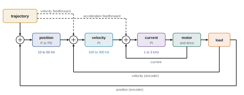
Almost every robot joint runs a cascade of three nested loops, each faster than the one around it:

• The current (torque) loop, usually a PI controller in the drive, runs at 10 to 40 kHz with a bandwidth of 1 to 3 kHz. It turns a current command into motor current despite back-EMF and winding inductance.
• The velocity loop, typically PI, runs at 2 to 10 kHz with a bandwidth of 100 to 300 Hz. It uses the encoder velocity and rejects friction and load disturbances.
• The position loop, typically P or PD with feedforward, runs at 1 to 4 kHz with a bandwidth of 10 to 50 Hz.

Each inner loop, closed and fast, looks to the outer loop like a near-ideal actuator: the velocity loop sees a torque source, the position loop sees a velocity source. The design rule is bandwidth separation, each loop five to ten times slower than the loop inside it, so the loops can be tuned one at a time from the inside out. Feedforward enters at every level: acceleration feedforward as a torque command to the current loop, velocity feedforward to the velocity loop. With a P position loop of gain \( K_v \) (in s⁻¹) around an ideal velocity loop, the following error at constant speed v without velocity feedforward is \( v/K_v \), which is why feedforward is essential for path accuracy.

Digital implementation

Controllers designed in continuous time must be discretized (ROB-230). For a PID, a standard form updates at each sample k with sample time h:

with the derivative usually filtered and taken on the measurement, and the integrator clamped for anti-windup. The Tustin (bilinear) transformation \( s \to \frac{2}{h}\frac{z - 1}{z + 1} \) preserves stability and is preferred for filters and lead compensators. Several implementation details matter as much as the control law:

• Sample rate: at least 10 to 20 times the closed-loop bandwidth; slower rates lose phase margin through the zero-order hold's delay of about h/2 (ROB-230).
• Latency: the time from sampling the encoder to applying the new torque adds to the loop delay. Good practice computes the output as early in the cycle as possible and applies it at a fixed instant.
• Jitter: variation in sample timing acts like noise on the time base. Real-time operating systems and hardware timers keep it to microseconds; general-purpose operating systems may not (ROB-320).
• Quantization: encoder resolution limits position measurement, and differencing quantized positions makes noisy velocity. High-resolution encoders, observers (lesson 6) or time-stamped edge counting help.
• Numeric format: integer or fixed-point arithmetic on small microcontrollers needs scaling to avoid overflow and to keep small integrator increments from being rounded away.