Trajectory tracking and computed torque control

With a smooth trajectory in hand, the controller's job is to make the robot follow it closely. Pure feedback, as in the PID loops of lesson 4, reacts only after an error has appeared; to follow a fast trajectory it needs a large error to generate the large torque the motion requires, so it always lags. The cure is to predict the torque the trajectory needs and apply it in advance, leaving feedback to correct only what the prediction gets wrong. This lesson develops that idea in stages: gravity compensation, which removes the steady sag of PD control; feedforward of the full dynamic model along the desired trajectory; and computed torque control, also called inverse dynamics control, which cancels the nonlinear dynamics so that every joint behaves like a simple, decoupled double integrator. It ends with what happens when the model is wrong, which it always is to some degree.

Why feedback alone lags

Consider a joint under PD control asked to follow \( q_d(t) = A\sin\omega t \). In steady state the torque required is roughly \( J\ddot{q}_d = -JA\omega^2\sin\omega t \), and a PD controller can only produce torque from error, \( \tau = K_pe + K_d\dot{e} \). The tracking error must therefore be about \( J\omega^2A/K_p \) in amplitude for low frequencies. Faster or larger motions mean larger errors, and raising the gains to shrink them is limited by stability, noise and resonances. Feedback is excellent at rejecting unpredictable disturbances; it is a poor way to generate predictable torques.

PD control with gravity compensation

The simplest model-based improvement adds the gravity vector to a PD law:

where \( \mathbf{e} = \mathbf{q}_d - \mathbf{q} \) for a constant target \( \mathbf{q}_d \). Gravity is now cancelled at every configuration, so there is no steady sag and no need for integral action to fight it. A classic result by Takegaki and Arimoto, published in 1981, shows that for any positive-definite diagonal gains this controller drives a rigid manipulator to any constant target from any initial state, using the energy-like function \( V = \tfrac{1}{2}\dot{\mathbf{q}}^{\mathsf{T}}\mathbf{M}\dot{\mathbf{q}} + \tfrac{1}{2}\mathbf{e}^{\mathsf{T}}\mathbf{K}_p\mathbf{e} \) and the skew-symmetry property of lesson 2. The proof never needs the inertia matrix or Coriolis terms to be known, only gravity. Gravity compensation is used in almost every industrial and collaborative robot; it is also what lets a collaborative arm be pushed around by hand in 'free drive' mode, where the controller cancels gravity and applies no position feedback at all.

Feedforward along the trajectory

For tracking, add the torque the desired trajectory needs, computed from the model by inverse dynamics, to a PD feedback law:

Because the feedforward depends only on the desired trajectory, it can be computed in advance, which is attractive when computation is limited. If the model is exact and the robot starts on the trajectory, the feedforward produces exactly the planned motion and the feedback has nothing to do. In practice it removes the bulk of the tracking error, and the feedback handles model error, friction and disturbances. Most industrial controllers use some form of this structure, often with friction feedforward added.

Computed torque control

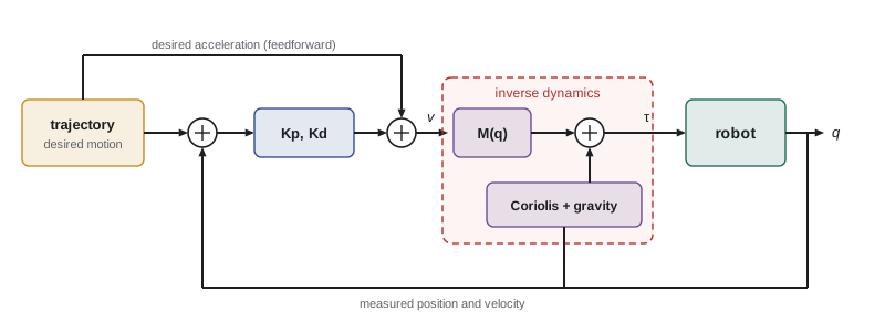
Computed torque control goes one step further: it evaluates the model at the actual state and uses it to cancel the nonlinear dynamics completely. Choose

Substituting into the manipulator equation \( \mathbf{M}\ddot{\mathbf{q}} + \mathbf{C}\dot{\mathbf{q}} + \mathbf{g} = \boldsymbol{\tau} \), the C and g terms cancel and, since M is invertible, \( \ddot{\mathbf{q}} = \mathbf{v} \). The closed loop becomes

a set of independent, linear, second-order error equations, one per joint, identical in every configuration and at every speed. With diagonal gains \( K_{p,i} = \omega_n^2 \) and \( K_{d,i} = 2\zeta\omega_n \), every joint's error decays like a critically damped spring whatever the arm is doing. Note that these gains are in units of acceleration, not torque: the inertia matrix scales them to torque automatically, which is why computed torque control needs no gain scheduling. The method is an example of feedback linearization: a nonlinear system made linear by a nonlinear feedback law.

The effect of model error

Computed torque control is only as good as its model. Suppose the controller uses estimates \( \hat{\mathbf{M}}, \hat{\mathbf{C}}, \hat{\mathbf{g}} \). The closed loop becomes

The mismatch acts as a disturbance η driving the otherwise perfect error dynamics. Small errors give small tracking errors, reduced further by high gains; large errors, such as an unmodelled payload, can degrade tracking badly. Friction is usually the largest unmodelled term and is added explicitly as a friction-compensation torque. Lesson 11 discusses robust and adaptive methods that keep performance despite model error. In practice, computed torque control is used with carefully identified models, and many industrial robots use the simpler feedforward form, which degrades more gracefully because it does not feed measured noise into the model terms.

Simulation: PD versus computed torque

The code below simulates the two-link arm following a quintic move of both joints, first with PD control plus gravity compensation (gains in torque units, scaled for the stretched-out arm), and then with computed torque control using the exact model. It reports the largest tracking error during the move.

import numpy as np
m1, m2, l1, lc1, lc2, I1, I2, g = 3, 2, 0.4, 0.2, 0.15, 0.04, 0.015, 9.81
a = I1 + I2 + m1*lc1**2 + m2*(l1**2 + lc2**2); b = m2*l1*lc2; d = I2 + m2*lc2**2
M = lambda q: np.array([[a + 2*b*np.cos(q[1]), d + b*np.cos(q[1])], [d + b*np.cos(q[1]), d]])
Cv = lambda q, qd: np.array([-b*np.sin(q[1])*(2*qd[0]*qd[1] + qd[1]**2), b*np.sin(q[1])*qd[0]**2])
G = lambda q: np.array([(m1*lc1 + m2*l1)*g*np.cos(q[0]) + m2*lc2*g*np.cos(q[0] + q[1]), m2*lc2*g*np.cos(q[0] + q[1])])
q0, qf, T = np.array([0.0, 0.5]), np.array([1.2, 1.8]), 1.0
def ref(t):
    s = min(t/T, 1.0); D = qf - q0
    return (q0 + D*(10*s**3 - 15*s**4 + 6*s**5), D/T*(30*s**2 - 60*s**3 + 30*s**4),
            D/T**2*(60*s - 180*s**2 + 120*s**3))
wn = 25.0
def run(mode, h=2e-4):
    q, qd, emax = q0.copy(), np.zeros(2), 0.0
    for k in range(int(1.5/h)):
        r, rd, rdd = ref(k*h); e, ed = r - q, rd - qd
        if mode == "pd":
            Mmax = M(np.zeros(2)).diagonal()
            tau = Mmax*wn**2*e + Mmax*2*wn*ed + G(q)
        else:
            tau = M(q) @ (rdd + 2*wn*ed + wn**2*e) + Cv(q, qd) + G(q)
        qdd = np.linalg.solve(M(q), tau - Cv(q, qd) - G(q))
        q, qd = q + h*qd, qd + h*qdd
        emax = max(emax, abs(e).max())
    return emax
print(f"PD + gravity:    max error {run('pd')*1000:7.2f} mrad")
print(f"computed torque: max error {run('ct')*1000:7.2f} mrad")

PD + gravity:    max error   43.74 mrad
computed torque: max error    0.06 mrad

With PD plus gravity compensation the arm lags its reference by tens of milliradians during the move, because feedback must generate the inertial and coupling torques from error. Computed torque control with an exact model tracks to within numerical integration error. Real results lie between: with a good identified model, computed torque or feedforward control typically cuts tracking error by a factor of five to twenty compared with PD alone.

Task-space control

Computed torque control can also be written in task space, where the error is the tool's position and orientation rather than joint angles. Khatib's operational-space formulation, from 1987, defines a task-space inertia \( \boldsymbol{\Lambda} = (\mathbf{J}\mathbf{M}^{-1}\mathbf{J}^{\mathsf{T}})^{-1} \) and computes joint torques \( \boldsymbol{\tau} = \mathbf{J}^{\mathsf{T}}\mathbf{F} \) from a task-space force F that cancels task-space dynamics. This makes the tool behave as a chosen mass-spring-damper in Cartesian space, which leads directly to the impedance control of lesson 10. For redundant robots, extra joint motions can be controlled in the null space of the Jacobian (ROB-210) without disturbing the tool.