
ROB-300 · Lesson 7 of 12 · 34 min
Optimal control: the linear quadratic regulator
Pole placement answers the question 'where should the poles go?' with the engineer's judgement, and for systems with many states and inputs that judgement becomes hard to exercise. Placing the four poles of a flexible joint is manageable; placing the twelve poles of a six-axis arm's linearized model, or of a balancing robot with several inputs, is not. The linear quadratic regulator, LQR, replaces pole locations with a more natural specification: a cost that penalizes state error and control effort, which the controller then minimizes. The result is a state-feedback gain with excellent robustness, computed reliably by software for systems of any size. LQR is used in balancing and legged robots, drones, satellite attitude control and as the inner layer of model predictive control. This lesson explains the cost function, the Riccati equation that solves it, how to choose the weights, and how to compute the gains numerically.
The quadratic cost
For the linear system \( \dot{\mathbf{x}} = \mathbf{A}\mathbf{x} + \mathbf{B}\mathbf{u} \), LQR finds the input that minimizes
The weighting matrix Q, symmetric and positive semidefinite, sets how much each state error costs; R, symmetric and positive definite, sets how much control effort costs. A large Q relative to R asks for aggressive control that drives errors to zero quickly at the price of large torques; a large R asks for gentle control that saves energy and avoids saturation at the price of slower response. The quadratic form is chosen partly for its mathematical convenience, but it also matches engineering intuition: small errors matter little, large errors matter a lot, and torque costs energy roughly in proportion to its square, since motor copper loss is \( i^2R \).
The solution: the Riccati equation
Remarkably, the optimal input for this infinite-horizon problem is a constant linear state feedback,
where P is the symmetric positive-definite solution of the continuous algebraic Riccati equation (CARE):
The matrix P has a physical meaning: the minimum achievable cost starting from state \( \mathbf{x}_0 \) is \( \mathbf{x}_0^{\mathsf{T}}\mathbf{P}\mathbf{x}_0 \). It acts as a cost-to-go, and it also serves as a Lyapunov function proving that the closed loop is stable. A solution exists and gives a stable closed loop when (A, B) is controllable (or at least stabilizable) and every unstable mode is penalized by Q (detectability). Only for small systems can the Riccati equation be solved by hand; normally it is solved numerically.
Worked problem
LQR for a first-order system
A motor speed loop is modelled as \( \dot{\omega} = -2\omega + 4u \). Find the LQR gain for Q = 10, R = 1, and the closed-loop pole.
Show solution
- Scalar CARE: \( 2ap - p^2b^2/r + q = 0 \) with a = −2, b = 4: \( -4p - 16p^2 + 10 = 0 \).
- Positive root: \( p = \frac{-4 + \sqrt{16 + 640}}{32} = \frac{-4 + 25.61}{32} = 0.675 \).
- Gain: \( k = bp/r = 4 \times 0.675 = 2.70 \).
- Closed-loop pole: \( a - bk = -2 - 10.8 = -12.8 \).
Answer: k = 2.70, moving the pole from −2 to −12.8. Raising Q to 100 would give k ≈ 9.0 and a pole near −38: heavier state weighting buys speed with effort. For a scalar system the closed-loop pole is always \( -\sqrt{a^2 + b^2q/r} \), so it depends only on the ratio q/r.
LQR for the double integrator
A lightly damped joint is close to a double integrator, \( \ddot{q} = u \) with u the torque divided by inertia. With \( \mathbf{Q} = \text{diag}(q_1, q_2) \) and scalar R = r, the Riccati equation can be solved in closed form, giving
so the closed-loop characteristic polynomial is \( s^2 + k_2s + k_1 \), with \( \omega_n = \sqrt{k_1} = (q_1/r)^{1/4} \) and, when \( q_2 = 0 \), \( \zeta = \sqrt{2}/2 \approx 0.707 \). Without any explicit request for damping, the optimal controller chooses a well-damped response with about 4 % overshoot. The fourth root means the weights must change a lot to change speed: multiplying \( q_1/r \) by 16 only doubles the natural frequency.
Worked problem
LQR gains for a joint
A joint with J = 1.5 kg·m² and negligible damping is to be controlled by LQR with u = τ/J, \( q_1 \) = 160,000, \( q_2 \) = 0 and r = 1. Find the gains in N·m units, \( \omega_n \) and ζ.
Show solution
- \( k_1 = \sqrt{160{,}000} = 400 \) s⁻²; \( k_2 = \sqrt{800} = 28.3 \) s⁻¹.
- \( \omega_n = \sqrt{400} = 20 \) rad/s; \( \zeta = 28.3/(2 \times 20) = 0.707 \).
- Torque gains: multiply by J: \( K_p = 600 \) N·m/rad, \( K_d = 42.4 \) N·m·s/rad.
Answer: \( K_p = 600 \) and \( K_d = 42.4 \), giving \( \omega_n \) = 20 rad/s with ζ = 0.707. Compared with the critically damped PD of lesson 4 (\( K_d \) = 59.5), LQR chooses less damping because it trades a little overshoot for lower control effort.
Choosing Q and R
The weights are the design knobs, and a systematic starting point is Bryson's rule: make each term in the cost roughly 1 when its variable reaches its largest acceptable value,
For a joint where an error of 0.01 rad and a torque of 50 N·m are each just tolerable, Bryson's rule gives \( Q_{11} = 10^4 \) and \( R = 4 \times 10^{-4} \). From there, tuning is iterative: simulate, look at the response and the peak torque, and scale the weights. Increase a state's weight if it settles too slowly or overshoots too much; increase R if the actuator saturates or the control is too noisy. Off-diagonal terms in Q can penalize combinations of states, such as the twist of a flexible joint, \( (\theta_1 - \theta_2)^2 \).
Worked problem
Bryson's rule for a balancing robot
A two-wheeled balancing robot has states: wheel position x (tolerable error 0.2 m), tilt θ (tolerable 0.05 rad), and their rates (tolerable 0.5 m/s and 0.5 rad/s). The wheel torque may reach 4 N·m. Write the Bryson weights.
Show solution
- \( Q = \text{diag}(1/0.2^2, 1/0.05^2, 1/0.5^2, 1/0.5^2) = \text{diag}(25, 400, 4, 4) \).
- \( R = 1/4^2 = 0.0625 \).
Answer: Q = diag(25, 400, 4, 4) and R = 0.0625. Tilt carries the largest weight because a small tilt is already dangerous for balance. These weights go into a numerical Riccati solver to produce the four feedback gains, which are then refined in simulation.
Robustness of LQR
LQR designs come with guaranteed robustness for single-input systems with full state feedback: a gain margin from 1/2 to infinity (the gain can be halved or increased without limit) and a phase margin of at least 60°. These guarantees follow from a property of the optimal loop called the return difference inequality, and they are one reason LQR is trusted in aerospace and robotics. The guarantees apply at the plant input and assume the full state is measured perfectly. When an observer supplies the state, as in lesson 6, the combined LQG design (LQR with a Kalman filter) can have arbitrarily poor margins, a famous result from 1978, so margins must be checked again; techniques such as loop transfer recovery address this.
Worked problem
Checking the guaranteed margin
For the double-integrator LQR of the joint example (k₁ = 400, k₂ = 28.3, in units of 1/J), compute the loop transfer function at the plant input and its phase margin.
Show solution
- Loop at the input: \( L(s) = \mathbf{K}(s\mathbf{I} - \mathbf{A})^{-1}\mathbf{B} = (k_2s + k_1)/s^2 = (28.3s + 400)/s^2 \).
- Crossover where \( |L(j\omega)| = 1 \): \( \sqrt{(28.3\omega)^2 + 400^2} = \omega^2 \). Solving \( \omega^4 - 800\omega^2 - 160{,}000 = 0 \) gives \( \omega^2 = 965.7 \), ω = 31.1 rad/s.
- Phase: \( -180° + \arctan(28.3 \times 31.1/400) = -180° + 65.5° \). Phase margin 65.5°.
Answer: About 65.5°, satisfying the guaranteed 60° minimum. The gain margin is infinite because the phase never reaches −180° at finite frequency.
Discrete-time LQR and the iterative Riccati solution
Robot controllers run in discrete time. For the sampled system \( \mathbf{x}_{k+1} = \mathbf{A}_d\mathbf{x}_k + \mathbf{B}_d\mathbf{u}_k \), obtained by exact discretization (ROB-230), the cost becomes a sum and the solution is \( \mathbf{u}_k = -\mathbf{K}\mathbf{x}_k \) with
where P solves the discrete algebraic Riccati equation. A simple, robust way to find P is to iterate the Riccati recursion backward from P = Q until it stops changing:
Each step of this recursion is one step of dynamic programming, solving the optimal control problem one more time step from the end. Run for a finite number of steps, it gives the finite-horizon LQR used inside model predictive control; run to convergence, it gives the constant infinite-horizon gain. In discrete time the cost weights are per sample, so Q and R from a continuous design should be scaled by the sample time h, roughly \( \mathbf{Q}_d \approx h\mathbf{Q} \) and \( \mathbf{R}_d \approx h\mathbf{R} \), to get similar behaviour.
import numpy as np
from math import sqrt
h = 0.001                                         # 1 kHz controller
Ad = np.array([[1, h], [0, 1]]); Bd = np.array([[h*h/2], [h]])   # exact ZOH double integrator
Q = np.diag([160000.0, 0.0])*h; R = np.array([[1.0]])*h
P = Q.copy()
for it in range(200000):
    G = np.linalg.solve(R + Bd.T @ P @ Bd, Bd.T @ P @ Ad)
    Pn = Q + Ad.T @ P @ Ad - Ad.T @ P @ Bd @ G
    if np.max(abs(Pn - P)) < 1e-9*np.max(abs(P)): break
    P = Pn
K = np.linalg.solve(R + Bd.T @ P @ Bd, Bd.T @ P @ Ad)
print(f"converged after {it} iterations; discrete K = {np.round(K, 2)}")
print(f"continuous formula: k1 = {sqrt(160000):.1f}, k2 = {sqrt(2*400):.2f}")
z = np.linalg.eigvals(Ad - Bd @ K); s = np.log(z)/h
wn = abs(s[0]); print(f"equivalent poles {np.round(s, 2)}, wn = {wn:.2f}, zeta = {-s[0].real/wn:.3f}")converged after 544 iterations; discrete K = [[394.38 28.08]] continuous formula: k1 = 400.0, k2 = 28.28 equivalent poles [-14.14+14.14j -14.14-14.14j], wn = 20.00, zeta = 0.707
The iteration converges in a few hundred steps to gains within about 1.5 % of the continuous closed-form result (394 against 400, and 28.1 against 28.3; the small difference comes from the sample-time scaling of the weights), and the equivalent continuous poles show the expected 20 rad/s natural frequency and damping ratio of 0.707. At 1 kHz the sampling barely matters for a 20 rad/s loop; for faster loops or slower controllers, the discrete design accounts for the sampling exactly where a continuous design would not.
LQR in robotics practice
Three practical patterns recur. First, LQR on a linearized model: balancing robots, quadrotors and legged robots in stance are linearized about an operating point (upright, hovering, standing) and stabilized by LQR, sometimes with gain scheduling across several operating points. Second, LQR around a trajectory: time-varying LQR, from the finite-horizon Riccati recursion along a planned motion, stabilizes deviations from a nominal trajectory computed by an optimizer. Third, LQR as the core of model predictive control (MPC), which re-solves a finite-horizon problem with explicit torque and state limits at every control step; LQR cannot handle such inequality constraints, MPC can, at higher computational cost. In all three, the cost weights are the main design interface, and the Bryson-rule starting point followed by simulation-based tuning is standard practice.
Worked problem
Effect of R on peak torque
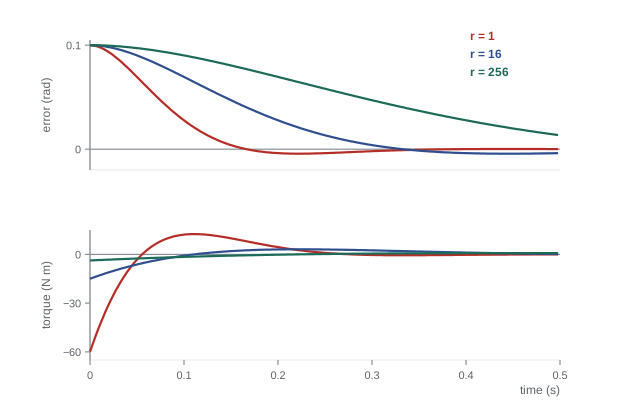
For the joint double-integrator LQR, an initial error of 0.1 rad at rest produces an initial torque \( Jk_1 \times 0.1 \). Compare the peak torque and natural frequency for r = 1 and r = 16 with \( q_1 \) = 160,000.
Show solution
- r = 1: \( k_1 = 400 \); initial torque \( 1.5 \times 400 \times 0.1 = 60 \) N·m; \( \omega_n \) = 20 rad/s.
- r = 16: \( k_1 = \sqrt{10{,}000} = 100 \); initial torque 15 N·m; \( \omega_n \) = 10 rad/s.
Answer: Multiplying R by 16 cuts the peak torque by a factor of 4 and halves the speed. If the motor can supply only 20 N·m, the larger R keeps the controller inside its limits, so it behaves as designed instead of saturating.
Common mistakes
MistakeExpecting large weight changes to give proportionally faster response
InsteadSpeed scales roughly with the fourth root of q/r for a double integrator; change weights by large factors.
MistakeUsing continuous Q and R unchanged in a discrete design
InsteadScale weights by the sample time, or design directly in discrete time.
MistakeAssuming LQR margins survive an observer
InsteadCheck margins again with the observer in the loop; LQG margins can be poor.
MistakeIgnoring actuator limits
InsteadIncrease R or use MPC so that peak torque stays inside the actuator envelope.
MistakeForgetting to penalize an unstable mode in Q
InsteadEvery unstable mode must be detectable through Q for a stabilizing solution.
Summary and key terms
- LQR minimizes \( \int(\mathbf{x}^{\mathsf{T}}\mathbf{Q}\mathbf{x} + \mathbf{u}^{\mathsf{T}}\mathbf{R}\mathbf{u})dt \), trading state error against control effort.
- The optimal control is \( \mathbf{u} = -\mathbf{R}^{-1}\mathbf{B}^{\mathsf{T}}\mathbf{P}\mathbf{x} \), with P from the algebraic Riccati equation.
- For a double integrator, \( k_1 = \sqrt{q_1/r} \) and \( k_2 = \sqrt{2k_1 + q_2/r} \), giving ζ = 0.707 when \( q_2 = 0 \).
- Bryson's rule sets initial weights from maximum acceptable state and input values.
- Single-input LQR with full state feedback guarantees at least 60° phase margin and a gain margin from 1/2 to infinity.
- Discrete LQR is found by iterating the Riccati recursion, which is dynamic programming backward in time.
- LQR stabilizes linearized robots and trajectories, and forms the core of model predictive control.
- Linear quadratic regulator
- The optimal state feedback for a linear system and quadratic cost.
- State weighting matrix
- The matrix Q penalizing state error in the cost.
- Control weighting matrix
- The matrix R penalizing control effort in the cost.
- Algebraic Riccati equation
- The matrix equation whose solution P gives the LQR gain.
- Cost-to-go
- The minimum remaining cost from a state, \( \mathbf{x}^{\mathsf{T}}\mathbf{P}\mathbf{x} \).
- Bryson's rule
- Choosing weights as the inverse squares of maximum acceptable values.
- Return difference
- The quantity 1 + L(jω) whose LQR properties guarantee robustness.
- LQG
- LQR combined with a Kalman filter state estimate.
- Riccati recursion
- The backward iteration that computes discrete LQR solutions.
- Model predictive control
- Repeatedly solving a finite-horizon optimal control problem with constraints.
Practice problems
Work each problem on paper first, then reveal the answer to check.
For \( \ddot{q} = u \), Q = diag(100, 0), r = 1, find \( k_1 \) and \( k_2 \).
Show answer
\( k_1 = 10 \), \( k_2 = \sqrt{20} = 4.47 \).
What damping ratio does that give?
Show answer
\( 4.47/(2\sqrt{10}) = 0.707 \).
By what factor must \( q_1/r \) rise to triple the natural frequency?
Show answer
\( 3^4 = 81 \).
Bryson's rule: maximum error 0.02 rad. What is \( Q_{11} \)?
Show answer
2,500.
Bryson's rule: maximum torque 10 N·m. What is R?
Show answer
0.01.
What is the scalar LQR pole for a = 0, b = 1, q = 25, r = 1?
Show answer
\( -\sqrt{25} = -5 \).
Name the guaranteed phase margin of single-input LQR.
Show answer
At least 60°.
Why might LQG have poor margins?
Show answer
The observer changes the loop; LQR guarantees assume measured states.
What can MPC do that LQR cannot?
Show answer
Enforce inequality constraints such as torque and joint limits.
What does each Riccati recursion step correspond to?
Show answer
One backward step of dynamic programming.
Lesson quiz · 5 questions
Score 60% or more to complete this lesson.
Create a free account to save your progress, take quizzes and earn a certificate.