
ROB-300 · Lesson 12 of 12 · 35 min
Capstone: designing and simulating a controller for a two-link arm
This capstone brings the whole course together on one realistic design problem. You will take a two-link arm from requirements to a simulated, verified controller: build its dynamic model, check that the motors can deliver the required torques, plan trajectories that respect the limits, choose a control structure and gains, account for friction, payload uncertainty, sampling and torque saturation, and test the design in simulation before it would ever run on hardware. The same workflow, scaled up with professional tools, is how robot motion control is engineered in industry. Each section below is a step in that workflow, with the calculations worked through for one design; a project brief at the end asks you to repeat it with your own choices.
Step 1: requirements
The robot is a planar two-link arm in a vertical plane, the arm used throughout this course: \( m_1 = 3 \) kg, \( m_2 = 2 \) kg, \( l_1 = 0.4 \) m, \( l_{c1} = 0.2 \) m, \( l_{c2} = 0.15 \) m, \( I_1 = 0.04 \) kg·m², \( I_2 = 0.015 \) kg·m², with a 0.3 m second link. It must move a part of up to 0.5 kg, carried at the end of link 2, between two configurations: from \( \mathbf{q}_A = [0, 0.5] \) rad to \( \mathbf{q}_B = [1.2, 1.8] \) rad. The requirements are:
- Move time no more than 1.0 s, followed by a 0.3 s settle, for a 1.3 s step of a repeating cycle.
- Tracking error during the move below 5 mrad on each joint, and final error below 0.5 mrad within 0.3 s of the end of the move.
- No overshoot of more than 0.5 mrad at the target (the part must not strike a fixture).
- Motor torque within limits at all times: 40 N·m at the shoulder and 12 N·m at the elbow, joint side, after gearing.
- Performance maintained with payload anywhere from 0 to 0.5 kg, with the controller not told the payload.
- Joint resonances, from harmonic drives, are at least 40 Hz (251 rad/s) at the shoulder and 60 Hz at the elbow.
Writing requirements as numbers matters: each will become a test in step 7. The tracking and overshoot limits set the controller type, the torque limits set the trajectory, and the resonances set the gain ceiling.
Step 2: model and parameters
From lesson 2, the inertia matrix, Coriolis and centrifugal vector and gravity vector of the arm are given by the constants α, β and δ, with the payload added as a point mass \( m_p \) at the tip of link 2 (distance \( l_2 = 0.3 \) m from the elbow). A point payload changes the link-2 parameters: its mass becomes \( m_2 + m_p \), its first moment \( m_2l_{c2} + m_pl_2 \) and its inertia about the elbow \( I_2 + m_2l_{c2}^2 + m_pl_2^2 \). Joint friction, from identification as in lesson 11, is modelled as Coulomb plus viscous: 1.0 N·m and 0.5 N·m·s/rad at the shoulder, 0.4 N·m and 0.2 N·m·s/rad at the elbow.
Worked problem
Payload effect on the model
Compute the shoulder and elbow inertias with the elbow at 90° (\( c_2 = 0 \)), and the shoulder gravity torque with both links horizontal, for payloads of 0 and 0.5 kg.
Show solution
- No payload: \( M_{11} = \alpha = 0.54 \), \( M_{22} = \delta = 0.06 \) kg·m² (lesson 2). Gravity with \( q_1 = q_2 = 0 \): \( g_1 = (0.6 + 0.8 + 0.3) \times 9.81 = 16.7 \) N·m.
- With 0.5 kg at 0.3 m from the elbow: δ rises by \( 0.5 \times 0.09 = 0.045 \) to 0.105; α rises by \( 0.5(0.16 + 0.09) = 0.125 \) to 0.665.
- Gravity: link-2 first moment rises by \( 0.5 \times 0.3 = 0.15 \), and link 2's mass at the elbow by 0.5 kg: \( g_1 \) rises by \( (0.5 \times 0.4 + 0.15) \times 9.81 = 3.43 \) to 20.1 N·m.
Answer: The payload raises the elbow inertia by 75 %, the shoulder inertia by 23 % and the worst-case shoulder gravity torque by about 20 %. The elbow is most sensitive, so the controller must cope with a large relative change there.
Step 3: trajectory and torque check
A synchronized quintic profile (lesson 8) moves both joints in exactly 1.0 s with zero velocity and acceleration at both ends, which helps keep the harmonic-drive resonances quiet. Joint 1 moves 1.2 rad and joint 2 moves 1.3 rad, so the peaks are \( 1.875\Delta/T \) in velocity and \( 5.77\Delta/T^2 \) in acceleration: 2.25 and 2.44 rad/s, and 6.9 and 7.5 rad/s². Before designing any controller, inverse dynamics along this trajectory with the heaviest payload gives the torques the motors must supply, and they must fit inside the limits with a margin for feedback correction, typically 20 to 30 %.
Worked problem
Peak torque and margin
Inverse dynamics along the trajectory with the 0.5 kg payload (computed in the code in step 6) gives peak torques of about 29 N·m at the shoulder and 6.8 N·m at the elbow, including gravity and friction. Check them against the limits and decide whether the move time is acceptable.
Show solution
- Shoulder margin: \( 1 - 29/40 = 27.5 \) %.
- Elbow margin: \( 1 - 6.8/12 = 43 \) %.
- Both exceed a 25 % target for feedback headroom, the shoulder only just.
Answer: The 1.0 s move fits, with 27.5 % shoulder and 43 % elbow margin. Had the shoulder needed 36 N·m, the move would need stretching; since a fair share of that torque is gravity, which does not scale with time (lesson 8), stretching would help less than expected.
Step 4: control structure and gains
Three structures are candidates. PD with gravity compensation is simple but lags during motion (lesson 9 found tens of milliradians), failing the 5 mrad requirement. Computed torque control with the nominal model tracks well but uses the model at the measured state, feeding encoder noise into the model terms. A practical choice, and the one chosen here, is feedforward of the nominal inverse dynamics along the desired trajectory plus PD feedback scaled by the nominal inertia, with gravity and friction compensation evaluated at the measured state, and a small integral term with anti-windup to remove residual steady error at the target:
where \( \hat{\mathbf{M}}_0 \) is the diagonal of the nominal inertia matrix at a mid-range configuration. Gains are set from the resonance limits: the shoulder resonance is 251 rad/s, so its feedback bandwidth should stay below about a third of that, roughly 80 rad/s. A natural frequency of 30 rad/s on both joints gives a comfortable margin while being fast enough to reject the model error caused by an unknown payload. Using the triple-pole PID rule from lesson 4 with ω = 30 rad/s, in acceleration units:
These are multiplied by the nominal inertias to give torque gains. The integrator is clamped to a few newton-metres and is the first place to look if the target overshoots.
Worked problem
Expected tracking error from payload mismatch
The controller assumes no payload. With the 0.5 kg payload the elbow inertia is 75 % larger than modelled. Estimate the elbow tracking error during the move, where the peak acceleration is 7.5 rad/s².
Show solution
- Unmodelled torque ≈ \( 0.045 \times 7.5 = 0.34 \) N·m inertial plus a gravity error up to \( 0.15 \times 9.81 = 1.47 \) N·m.
- With feedback stiffness \( \hat{M}_{22}K_p = 0.06 \times 2700 = 162 \) N·m/rad, the quasi-static error is roughly \( (0.34 + 1.47)/162 = 0.011 \) rad.
- The integral term removes the slowly varying gravity part over a fraction of a second, so the peak during the move will be several mrad, decaying toward zero.
Answer: Roughly 5 to 10 mrad at the elbow if the payload gravity is not compensated, at or above the 5 mrad limit. The design therefore either needs payload identification (lesson 11) or relies on the integrator acting fast enough; the simulation below checks which.
Step 5: discrete implementation and limits
The controller runs at 1 kHz with one sample of computation delay, a realistic rate for a joint controller. From lesson 11, the zero-order hold and one-sample delay add about 1.5 ms of effective delay, costing \( 30 \times 0.0015 = 0.045 \) rad, or 2.6°, of phase at the 30 rad/s bandwidth: negligible. Velocity comes from a filtered difference of encoder positions with 0.1 mrad resolution (about 16 bits per revolution after gearing). Torques are saturated at the joint limits, with back-calculation anti-windup on the integrator.
Step 6: simulation
The simulation below integrates the true arm, with payload and friction, using small RK4 steps, while the controller runs at 1 kHz on quantized position measurements and holds its torque between updates. It first computes the inverse-dynamics torque along the path, then runs the cycle three times: with no payload, with the 0.5 kg payload unknown to the controller (which keeps the no-payload model), and with the payload identified so the controller's model includes it. Velocity is a filtered difference of the quantized positions.
import numpy as np
g, l1, l2 = 9.81, 0.4, 0.3
def params(mp):
    m1, m2, lc1, lc2, I1, I2 = 3, 2, 0.2, 0.15, 0.04, 0.015
    m2e = m2 + mp; mlc2 = m2*lc2 + mp*l2; I2o = I2 + m2*lc2**2 + mp*l2**2   # link 2 with payload
    a = I1 + m1*lc1**2 + m2e*l1**2 + I2o; b = l1*mlc2; d = I2o
    return a, b, d, (m1*lc1 + m2e*l1)*g, mlc2*g
def M(p, q): a, b, d, _, _ = p; c = np.cos(q[1]); return np.array([[a + 2*b*c, d + b*c], [d + b*c, d]])
def Cv(p, q, w): b = p[1]; s = np.sin(q[1]); return np.array([-b*s*(2*w[0]*w[1] + w[1]**2), b*s*w[0]**2])
def G(p, q): return np.array([p[3]*np.cos(q[0]) + p[4]*np.cos(q[0]+q[1]), p[4]*np.cos(q[0]+q[1])])
Fc, B = np.array([1.0, 0.4]), np.array([0.5, 0.2])
fric = lambda w: Fc*np.tanh(w/0.01) + B*w
qA, qB, T = np.array([0.0, 0.5]), np.array([1.2, 1.8]), 1.0
def ref(t):
    s = min(max(t/T, 0), 1); D = qB - qA
    return qA + D*(10*s**3-15*s**4+6*s**5), D/T*(30*s**2-60*s**3+30*s**4), D/T**2*(60*s-180*s**2+120*s**3)
w0 = 30.0; Kp, Kd, Ki = 3*w0**2, 3*w0, w0**3
tlim = np.array([40.0, 12.0]); res = 1e-4
def run(mp, mp_model, h=1e-4, dt=1e-3):
    tru, nom = params(mp), params(mp_model); M0 = M(nom, np.array([0.6, 1.15])).diagonal()
    q, w = qA.copy(), np.zeros(2)
    integ, tau, tau_next, qprev, wf = np.zeros(2), np.zeros(2), np.zeros(2), qA.copy(), np.zeros(2)
    emove, epk_tau, eend, overs = 0.0, np.zeros(2), 0.0, 0.0
    per = int(round(dt/h))
    for k in range(int(1.3/h)):
        t = k*h
        if k % per == 0:
            tau = tau_next                                    # apply last sample's result (one-sample delay)
            qm = np.round(q/res)*res; wf += 0.25*((qm - qprev)/dt - wf); qprev = qm   # filtered velocity
            r, rd, rdd = ref(t); e, ed = r - qm, rd - wf
            ff = M(nom, r) @ rdd + Cv(nom, r, rd) + G(nom, qm) + fric(rd)
            u = ff + M0*(Kp*e + Kd*ed + Ki*integ)
            tau_next = np.clip(u, -tlim, tlim)
            integ += dt*(e + (tau_next - u)/(M0*Ki*0.05))
        acc = np.linalg.solve(M(tru, q), tau - Cv(tru, q, w) - G(tru, q) - fric(w))
        q, w = q + h*w, w + h*acc
        r = ref(t)[0]; err = abs(r - q)
        if t <= T: emove = max(emove, err.max())
        else:
            overs = max(overs, ((q - qB)*np.sign(qB - qA)).max())
        epk_tau = np.maximum(epk_tau, abs(tau))
    eend = abs(qB - q).max()
    return emove, eend, overs, epk_tau
p5 = params(0.5)                                          # inverse dynamics along the path, heavy payload
tid = np.max([abs(M(p5, r) @ rdd + Cv(p5, r, rd) + G(p5, r) + fric(rd))
              for r, rd, rdd in (ref(t) for t in np.linspace(0, T, 2001))], axis=0)
print("inverse-dynamics peak torque with 0.5 kg (N m):", np.round(tid, 1))
for mp, mm, label in ((0.0, 0.0, "no payload"), (0.5, 0.0, "0.5 kg, unknown"), (0.5, 0.5, "0.5 kg, identified")):
    em, ee, ov, tp = run(mp, mm)
    print(f"{label:18s}: move error {em*1e3:5.2f} mrad, final {ee*1e3:5.3f} mrad, "
f"overshoot {max(ov,0)*1e3:5.3f} mrad, peak torque {np.round(tp,1)} N m")inverse-dynamics peak torque with 0.5 kg (N m): [29. 6.8] no payload : move error 0.70 mrad, final 0.142 mrad, overshoot 0.386 mrad, peak torque [24.7 4.7] N m 0.5 kg, unknown : move error 9.18 mrad, final 0.341 mrad, overshoot 0.151 mrad, peak torque [30.5 7.1] N m 0.5 kg, identified: move error 0.75 mrad, final 0.053 mrad, overshoot 0.400 mrad, peak torque [30.3 7.1] N m
The results are compared with the requirements in the next step. Observe how much of the code is not the control law: the true model with payload, the friction, the quantized measurement, the one-sample delay, the torque limits and the anti-windup. A simulation that leaves these out flatters the design.
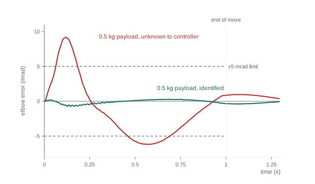
Step 7: verification against requirements
Each requirement from step 1 becomes a pass or fail check. The table records the outcome for this design, using the simulation output.
| Requirement | Limit | No payload | 0.5 kg payload | Result |
|---|---|---|---|---|
| Tracking error during move | 5 mrad | 0.70 | 9.18 (unknown) / 0.75 (identified) | Fails unless payload identified |
| Final error 0.3 s after move | 0.5 mrad | 0.14 | 0.34 / 0.05 | Pass |
| Overshoot at target | 0.5 mrad | 0.39 | 0.15 / 0.40 | Pass |
| Peak shoulder torque | 40 N·m | 24.7 | 30.5 / 30.3 | Pass |
| Peak elbow torque | 12 N·m | 4.7 | 7.1 / 7.1 | Pass |
| Feedback bandwidth vs resonance | < 84 rad/s | 30 rad/s | 30 rad/s | Pass |
Without a payload, every requirement passes with margin. With the 0.5 kg payload unknown to the controller, the move error reaches about 9 mrad, inside the range predicted in step 4 and nearly twice the limit, mainly from the uncompensated payload gravity and inertia at the elbow; the integrator then removes most of it during the settle, so the final-error and overshoot requirements still pass. With the payload identified and included in the model, the move error returns to under 1 mrad. The design therefore passes only with payload identification, which becomes a requirement on the robot's software. Note also that the commanded peak torques stay close to the pure inverse-dynamics values, because the feedback adds little when the feedforward is accurate. When a requirement fails, the options in order of preference are: improve the model (identify the payload at pick-up and update the feedforward), raise the bandwidth within the resonance limit, add a disturbance observer, or relax the requirement with the customer. Changing the trajectory to a longer move time is a last resort because it costs cycle time.
Worked problem
Interpreting a failed requirement
The unknown 0.5 kg payload gave a move error of 9.2 mrad. Using the scaling ideas of lesson 11, what bandwidth would bring it under 5 mrad without payload identification, and is that allowed?
Show solution
- Model-error tracking error scales roughly with \( 1/\omega_n^2 \).
- Required ratio: \( \sqrt{9.2/5} = 1.36 \); new bandwidth ≈ 30 × 1.36 = 41 rad/s.
- Elbow resonance is 60 Hz = 377 rad/s; a third of that is 126 rad/s, so 40 rad/s is allowed. The shoulder limit, 84 rad/s, is also respected.
Answer: Raising the natural frequency to about 41 rad/s, or a little more for margin, should bring the error under 5 mrad, and it stays well inside both resonance limits. Payload identification would still be the better fix, because it removes the error at its source and keeps the gains, and so the noise sensitivity, lower.
Step 8: from simulation to hardware
A design that passes in simulation is ready for careful hardware testing, not for production. The usual sequence is to verify the current loops and encoder directions with the arm disconnected or blocked; run gravity compensation alone and check the arm floats when pushed; close the joint loops with low gains, then raise them while watching for resonance, using a frequency sweep to measure the real resonances and margins; identify the dynamic parameters with exciting trajectories; enable feedforward and compare tracking with the simulation; and finally run the production cycle with all payloads and at temperature extremes, since friction changes with temperature. Safety functions, such as torque and speed limits, collision detection by comparing measured and modelled torques, and safe stopping, are configured and tested alongside, following the standards introduced in ROB-450.
Project brief
Repeat the design for your own variation and document each step:
- Change one requirement: for example a 0.7 s move, a 2 kg payload or a 25 Hz shoulder resonance. Recompute the peak torques and decide whether the motors still suffice.
- Choose a trajectory type (quintic, trapezoidal or S-curve) and justify it against the resonances and torque limits.
- Choose and justify a control structure and gains, showing the resonance and phase-margin checks.
- Modify the simulation code to model your case, including friction, quantization, delay and torque limits, and add payload identification or a disturbance observer if your requirements demand it.
- Fill in the verification matrix with your simulation results, and write a short hardware test plan in the order given in step 8.
A good report shows not just that the design works but why: which requirement drove each decision, and how much margin remains on each check.
Common mistakes
MistakeDesigning the controller before checking that the motors can deliver the trajectory
InsteadRun inverse dynamics along the trajectory first and keep 20 to 30 % torque margin.
MistakeSimulating without friction, quantization, delay and torque limits
InsteadInclude the real non-idealities, or the simulation will flatter the design.
MistakeChoosing gains without reference to resonances
InsteadKeep feedback bandwidth below about a third of the lowest resonance.
MistakeTesting only the nominal payload
InsteadVerify the full payload range and temperature range.
MistakeTreating requirements as qualitative
InsteadState each as a number and turn it into a pass or fail test.
Summary and key terms
- A control design starts from numerical requirements on time, accuracy, overshoot, torque and robustness.
- The dynamic model, including payload and friction, quantifies how much the plant varies.
- Inverse dynamics along the planned trajectory checks torque limits before any controller is designed.
- Feedforward of nominal dynamics plus inertia-scaled PID feedback is a robust, practical structure.
- Gains are bounded by resonances; delay and sampling are checked in the phase budget.
- Simulation with realistic non-idealities verifies every requirement in a verification matrix.
- Hardware commissioning proceeds inside-out, from current loops to the full cycle, with safety functions tested alongside.
- Requirement
- A measurable statement of what the system must achieve.
- Verification matrix
- A table mapping each requirement to its test and result.
- Torque margin
- The fraction of actuator torque left for feedback after feedforward needs.
- Nominal model
- The model used by the controller, typically without payload.
- Payload identification
- Estimating payload mass and centre of mass from motion and torque data.
- Commissioning
- Bringing a controller into operation on hardware step by step.
- Frequency sweep
- Exciting a system across frequencies to measure its response, resonances and margins.
- Collision detection
- Detecting unexpected contact by comparing measured and modelled torques.
- Cycle time
- The time for one complete repetition of a task.
- Headroom
- Spare capability kept in reserve for disturbances and model error.
Practice problems
Work each problem on paper first, then reveal the answer to check.
A 0.5 kg payload at 0.3 m adds what to the elbow inertia?
Show answer
0.045 kg·m².
Quintic move of 1.3 rad in 1.0 s: peak velocity?
Show answer
About 2.44 rad/s.
Peak torque 30 N·m against a 40 N·m limit: margin?
Show answer
25 %.
Shoulder resonance 251 rad/s. Maximum sensible feedback bandwidth?
Show answer
About 80 rad/s.
PID triple-pole gains in acceleration units for ω = 20 rad/s?
Show answer
\( K_d = 60 \), \( K_p = 1200 \), \( K_i = 8000 \).
Phase cost of 1.5 ms delay at 30 rad/s?
Show answer
About 2.6°.
Name two non-idealities a realistic simulation must include.
Show answer
Friction, quantization, delay, torque limits or payload error.
A tracking error of 8 mrad must fall to 4 mrad by raising bandwidth. By what factor?
Show answer
About \( \sqrt{2} = 1.41 \).
What is the first hardware test after current loops?
Show answer
Gravity compensation alone, checking the arm floats.
Why identify the payload rather than raise gains?
Show answer
It removes the error at its source and keeps noise sensitivity and resonance risk lower.
Lesson quiz · 5 questions
Score 60% or more to complete this lesson.
Create a free account to save your progress, take quizzes and earn a certificate.