Information filters, smoothing and factor graphs

The filters so far estimate only the current state and forget the past: once a measurement has been folded into the belief, it is never revisited. This is efficient, but it throws away the chance to improve old estimates with new information, and it locks in linearization errors made with poor estimates. Modern robotics increasingly uses smoothing instead, estimating the whole trajectory, or a recent window of it, from all the measurements at once, by solving a sparse nonlinear least-squares problem represented as a factor graph. This lesson builds the bridge from filtering to smoothing: first the information form of the Gaussian, in which fusion is simple addition; then batch least-squares estimation; then factor graphs and the sliding-window and incremental methods that make smoothing run in real time. These ideas are the foundation of the graph-based SLAM covered in ROB-340 and of most current visual-inertial and lidar odometry systems.

The information form

A Gaussian can be written with its covariance Σ and mean μ, the moment form, or with the information matrix \( \boldsymbol{\Omega} = \boldsymbol{\Sigma}^{-1} \) and information vector \( \boldsymbol{\xi} = \boldsymbol{\Omega}\boldsymbol{\mu} \), the canonical or information form. The two describe the same distribution, but they make different operations easy. In the information form, the measurement update of a Kalman filter becomes addition:

Each measurement contributes its own information, independent of the others, and fusing many sensors means summing their contributions, the matrix version of the inverse-variance addition of lesson 5. A complete absence of knowledge is easy to represent too: Ω = 0, which in moment form would need an infinite covariance. The price is that prediction, simple in moment form, becomes awkward in information form, and recovering the mean requires solving \( \boldsymbol{\Omega}\boldsymbol{\mu} = \boldsymbol{\xi} \). The information filter is therefore used where measurement updates dominate, such as fusing many sensors at once or decentralized estimation across several robots, where each robot can simply send its information contribution to the others.

Sparsity and the structure of robot problems

The information matrix reveals the structure of an estimation problem. Its off-diagonal entry between two variables is zero if and only if they are conditionally independent given all the other variables; equivalently, nonzero entries appear only between variables directly linked by some measurement or motion constraint. For a robot trajectory, pose \( x_t \) is directly linked only to \( x_{t-1} \) and \( x_{t+1} \) by odometry, and to the landmarks it observed. The information matrix of a full trajectory is therefore sparse: banded along the diagonal, with extra entries only for observations. The covariance matrix, in contrast, is dense, because every pose is indirectly correlated with every other through the chain. Sparse matrices can be stored and factorized in time roughly proportional to the number of nonzero entries rather than to the cube of the dimension, which is what makes estimating thousands of poses at once feasible.

From filtering to smoothing

Filtering estimates \( p(x_t \mid z_{1:t}) \), the current state from all data so far. Smoothing estimates \( p(x_{0:t} \mid z_{1:t}) \), the whole trajectory, so that a measurement at time t can also improve the estimate of where the robot was at time t − 10. For a linear Gaussian system, the forward Kalman filter followed by a backward Rauch–Tung–Striebel pass gives the exact smoothed estimates; past states benefit from future measurements and their uncertainty shrinks. For nonlinear systems, smoothing has a further advantage: it can re-linearize past models around improved estimates, removing the linearization errors that a filter locks in forever.

The modern way to compute a smoothed estimate is as a maximum a posteriori (MAP) problem. With Gaussian noise, maximizing the posterior of the trajectory is equivalent to minimizing a sum of squared, covariance-weighted residuals, one for each motion constraint, measurement and prior:

Here \( \mathbf{r}_k \) is the difference between what model k predicts and what was measured, such as odometry predicting \( x_t - x_{t-1} \) and measuring \( u_t \). Gauss–Newton solves this by repeatedly linearizing the residuals with their Jacobian J and solving the normal equations \( (\mathbf{J}^{\mathsf{T}}\mathbf{W}\mathbf{J})\Delta\mathbf{X} = -\mathbf{J}^{\mathsf{T}}\mathbf{W}\mathbf{r} \), where W holds the inverse covariances. The matrix \( \mathbf{J}^{\mathsf{T}}\mathbf{W}\mathbf{J} \) is exactly the information matrix of the trajectory, sparse for the reasons above. Levenberg–Marquardt adds damping for robustness when the starting estimate is poor.

Factor graphs

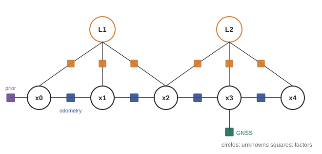
A factor graph draws the least-squares problem as a bipartite graph. Variable nodes represent unknowns: robot poses, landmark positions, sensor biases, calibration parameters. Factor nodes represent the terms of the cost: a prior factor attached to the first pose, odometry factors between consecutive poses, measurement factors between a pose and a landmark, a GNSS factor on a single pose, an IMU preintegration factor linking two poses and their velocities and biases. The graph makes the sparsity visible, it makes the problem modular (adding a new sensor means defining a new kind of factor), and it maps directly onto efficient solvers. Libraries such as GTSAM, Ceres Solver and g2o are built around this abstraction, and most state-of-the-art odometry and SLAM systems, including visual-inertial systems like VINS-Mono and lidar systems like LIO-SAM, are factor-graph smoothers.

import numpy as np
rng = np.random.default_rng(12)
T, so, sb = 50, 0.05, 0.3                     # 50 steps, odometry noise, beacon noise
fix_times = range(10, T + 1, 10)              # beacon every 10 steps
def trial():
    true = np.cumsum(np.r_[0.0, np.full(T, 0.5)])
    u = np.diff(true) + rng.normal(0, so, T)                    # noisy odometry
    beac = {t: true[t] + rng.normal(0, sb) for t in fix_times}
    mu, P, filt = 0.0, 0.01, [0.0]                              # forward Kalman filter (1-D)
    for t in range(1, T + 1):
        mu, P = mu + u[t - 1], P + so**2
        if t in beac: K = P/(P + sb**2); mu, P = mu + K*(beac[t] - mu), (1 - K)*P
        filt.append(mu)
    rows, rhs, w = [np.eye(T + 1)[0]], [0.0], [1/0.1**2]        # batch least squares: prior,
    for t in range(1, T + 1):                                   # odometry factors,
        rows.append(np.eye(T + 1)[t] - np.eye(T + 1)[t - 1]); rhs.append(u[t - 1]); w.append(1/so**2)
    for t, z in beac.items():                                   # and beacon factors
        rows.append(np.eye(T + 1)[t]); rhs.append(z); w.append(1/sb**2)
    J, r, W = np.array(rows), np.array(rhs), np.diag(w)
    Om = J.T @ W @ J; smooth = np.linalg.solve(Om, J.T @ W @ r)
    rmse = lambda est: np.sqrt(np.mean((np.array(est) - true)**2))
    return rmse(filt), rmse(smooth), np.count_nonzero(Om)
res = np.array([trial() for _ in range(300)])
print(f"mean RMSE over 300 runs: filter {res[:, 0].mean():.3f} m, smoother {res[:, 1].mean():.3f} m")
print(f"smoother better in {np.mean(res[:, 1] < res[:, 0])*100:.0f} % of runs")
print(f"information matrix nonzeros: {int(res[0, 2])} of {(T + 1)**2}")

mean RMSE over 300 runs: filter 0.179 m, smoother 0.144 m
smoother better in 73 % of runs
information matrix nonzeros: 151 of 2601

Averaged over 300 simulated runs, the smoother's error over the whole trajectory is about 20 % lower than the filter's (0.144 m against 0.179 m), because each beacon fix corrects the poses before it as well as after it, while the filter's estimates of past poses keep the drift they had at the time. In any single run the noise can favour either method, which is why estimators are compared over many runs, but the smoother wins in about three runs out of four. The information matrix has only about three nonzeros per row, a tridiagonal band, so even this naive dense solve could be replaced by a banded solver whose cost grows linearly with trajectory length.

Real-time smoothing

A full smoother re-solving the entire history at every step would eventually become too slow. Two techniques keep smoothing real-time. Fixed-lag or sliding-window smoothing keeps only the most recent N poses (often 10 to 50) as variables and marginalizes older ones out, summarizing their effect as a prior on the oldest remaining pose. Marginalization in information form is computed with the Schur complement; it preserves the information from old measurements but turns their linearization into a fixed approximation and creates fill-in, new nonzeros linking all the variables that were connected to the removed ones. Most visual-inertial odometry systems use this approach. Incremental smoothing, exemplified by iSAM2 in GTSAM, keeps the whole graph but updates the factorization of the information matrix incrementally as new factors arrive, re-linearizing only the variables whose estimates have changed significantly. It gives the accuracy of a full batch solution at a cost close to that of a filter for most steps, with occasional larger updates, for example when a loop closure in SLAM connects the current pose to one seen long ago.