The Bayes filter and histogram localization

Lesson 1 showed how a single measurement updates a belief through Bayes' rule. A robot, however, does not take one measurement and stop: it moves, senses, moves again and senses again, hundreds of times a second. The Bayes filter is the recursive algorithm that keeps a belief up to date through this cycle, alternating a prediction step, which accounts for motion, with a correction step, which accounts for each new measurement. Every estimator in this course, from the Kalman filter to the particle filter, is an implementation of the Bayes filter with a particular way of representing the belief. This lesson derives the filter, explains the Markov assumption that makes it recursive, and implements it exactly for a robot in a one-dimensional corridor using a histogram, a representation simple enough to compute by hand.

The recursive estimation problem

The robot wants its belief \( bel(x_t) = p(x_t \mid z_{1:t}, u_{1:t}) \), the distribution of its current state given every measurement and control so far. Computing this directly from the full history would get slower and slower as the history grows. The Bayes filter instead computes \( bel(x_t) \) from \( bel(x_{t-1}) \), the latest control \( u_t \) and the latest measurement \( z_t \), so that each update costs the same no matter how long the robot has been running. The previous belief is a sufficient summary of everything that came before.

Two assumptions make this possible, together called the Markov assumption. First, the state is complete: given the current state, the future measurement depends on nothing else from the past, \( p(z_t \mid x_{0:t}, z_{1:t-1}, u_{1:t}) = p(z_t \mid x_t) \). Second, given the previous state and the current control, the current state does not depend on older history, \( p(x_t \mid x_{0:t-1}, z_{1:t-1}, u_{1:t}) = p(x_t \mid x_{t-1}, u_t) \). In words, the state captures everything about the past that matters for predicting the future. This is an idealization. Unmodelled effects such as a slowly drifting gyro bias, people moving through the scene, or a wheel that slips repeatedly on the same patch of floor make errors correlated over time and violate the assumption. The usual remedies are to add the hidden quantity to the state (estimating the gyro bias along with the pose, for example), to inflate noise models so the filter stays cautious, or to reject measurements that do not fit.

Prediction and correction

Under the Markov assumption, the Bayes filter is two equations. The prediction step uses the law of total probability to push the previous belief through the motion model:

For every possible current state, it adds up the probability of having come from each possible previous state. Prediction spreads the belief out, because motion is uncertain: a robot that was fairly sure where it was becomes less sure after driving with slipping wheels. The correction step, or measurement update, applies Bayes' rule with the measurement model:

It multiplies the predicted belief by the likelihood of the measurement at each state and normalizes. Correction usually sharpens the belief, concentrating probability on states consistent with what the sensor saw. A robot running a Bayes filter alternates between these steps, and the shape of its belief breathes in and out: wider after each motion, narrower after each informative measurement. If no measurement arrives, the robot simply keeps predicting, and the belief keeps spreading, which is exactly the right behaviour for dead reckoning.

Representing the belief as a histogram

The Bayes filter equations are exact but involve integrals over continuous states, which cannot be computed in general. The histogram filter makes them computable by dividing the state space into a finite number of cells and storing one probability per cell. The integral in the prediction step becomes a sum, and the correction step becomes an element-wise multiplication followed by normalization:

Histograms can represent any shape of belief, including several separate peaks, which is their great strength. Their weakness is cost: the number of cells grows exponentially with the dimension of the state. A one-dimensional corridor with 1,000 cells is trivial; a planar pose with 10 cm cells over a 50 m by 50 m building and 1° heading bins has 250,000 × 360 = 90 million cells. Histogram filters are therefore used for low-dimensional problems or coarse global localization, while higher-dimensional problems use Gaussians (lessons 5 to 7) or samples (lesson 8).

A corridor example

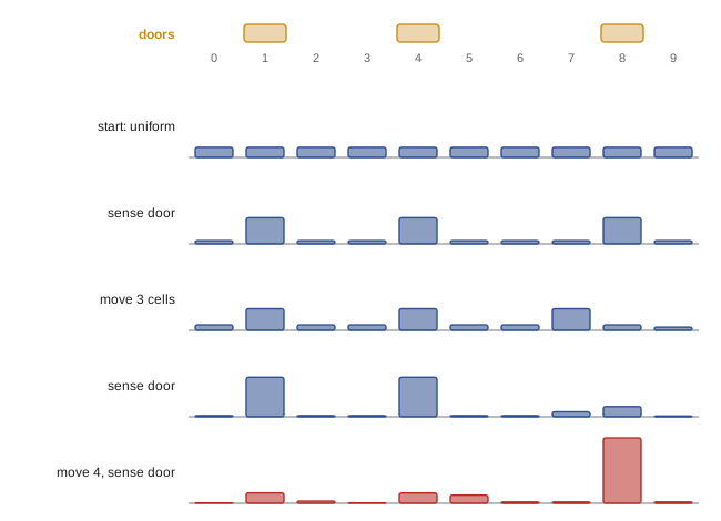
Consider a robot in a corridor of ten cells, numbered 0 to 9, with doors in front of cells 1, 4 and 8. The robot has a door detector that reports "door" with probability 0.8 when it is in front of a door and with probability 0.1 otherwise. When commanded to move one cell to the right, it actually moves one cell with probability 0.8, stays put with probability 0.1 and overshoots by two cells with probability 0.1. The corridor wraps around for simplicity, so moving right from cell 9 leads to cell 0. Initially the robot has no idea where it is: the belief is uniform, 0.1 in each cell.

After the move, the three peaks sit at cells 2, 5 and 9, each a little lower and wider. None of those cells has a door, so a "no door" reading would now be expected, and it would leave the three hypotheses roughly balanced. The interesting case is a sequence of moves that carries one hypothesis onto another door while the others land on blank wall. Whichever hypothesis predicts the observed sequence of doors and walls accumulates probability, and the others fade. After a few cycles in a corridor with an irregular door pattern, one peak dominates and the robot has localized itself globally, starting from total ignorance.

import numpy as np
doors = np.zeros(10); doors[[1, 4, 8]] = 1
def sense(bel, z):                       # z = 1 means "door"
    like = np.where(doors == 1, 0.8, 0.1) if z else np.where(doors == 1, 0.2, 0.9)
    b = like * bel; return b / b.sum()
def move(bel, u):                        # move u cells right, with slip
    return 0.8*np.roll(bel, u) + 0.1*np.roll(bel, u - 1) + 0.1*np.roll(bel, u + 1)
bel = np.full(10, 0.1)
for z, u in [(1, 3), (1, 4), (1, 0)]:    # sense door, move 3, sense door, move 4, sense door
    bel = sense(bel, z)
    print("after sensing", "door   " if z else "no door", np.round(bel, 3))
    if u: bel = move(bel, u)
print("most likely cell:", int(np.argmax(bel)), " probability:", round(float(bel.max()), 3))

after sensing door    [0.032 0.258 0.032 0.032 0.258 0.032 0.032 0.032 0.258 0.032]
after sensing door    [0.013 0.39  0.013 0.013 0.39  0.013 0.013 0.049 0.101 0.007]
after sensing door    [0.004 0.103 0.022 0.004 0.102 0.081 0.013 0.013 0.645 0.013]
most likely cell: 8  probability: 0.645

The code moves the robot three cells and then four cells between sightings. Of the three initial hypotheses (cells 1, 4 and 8), only the one starting at cell 1 sees doors at every sighting (1, then 4, then 8); the one starting at cell 8 matches twice (8, then 1) before landing on blank wall at cell 5, so its probability grows at every step while the others fall. After the second sighting the belief has two equal peaks of 0.39 at cells 1 and 4 (the hypothesis from cell 8 also landed on a door, at cell 1), and after the third it puts about 65 % of its probability on cell 8, with most of the rest spread over the overshoot and undershoot paths. A fourth or fifth sighting would push it above 90 %. The robot localized itself using only a crude binary sensor and noisy motion, because the pattern of doors along its path is distinctive. Corridors with perfectly regular door spacing would never allow this, a real issue in symmetric buildings where robots need extra cues such as signs, Wi-Fi fingerprints or room numbers.

Practical issues

Several practical matters arise even in this simple filter. Probabilities can underflow to zero after many multiplications, so implementations normalize after every update and often work with log-probabilities, where products become sums. A cell whose probability reaches exactly zero can never recover, even if the robot is actually there, so filters keep a small floor probability or inject a little uniform probability each step to recover from mistakes; lesson 8 calls this the kidnapped robot problem. The cell size is a design trade-off: cells that are too large lose precision, while cells that are too small make the filter slow and can cause motion updates to spread probability poorly if the motion per step is less than one cell. Finally, the filter is only as good as its models: if the door detector actually reports false doors 30 % of the time but the filter assumes 10 %, the belief will become overconfident and may lock onto the wrong cell.