
ROB-310 · Lesson 7 of 12 · 29 min
The unscented Kalman filter and comparing Gaussian filters
The extended Kalman filter approximates a nonlinear function by its tangent, which requires derivatives and ignores curvature. The unscented Kalman filter, UKF, introduced by Simon Julier and Jeffrey Uhlmann in the 1990s, takes a different view: it is easier to approximate a probability distribution than an arbitrary nonlinear function. Instead of linearizing, the UKF picks a small, deterministic set of sample points, called sigma points, that capture the mean and covariance of the belief, passes each one through the true nonlinear function, and recomputes a mean and covariance from the transformed points. No Jacobians are needed, and the result captures second-order effects that the EKF misses. This lesson explains the unscented transform, builds the UKF from it, and then compares the EKF, UKF and the particle filters of the next lesson so that you can choose sensibly among them.
The unscented transform
For an n-dimensional Gaussian with mean μ and covariance Σ, the standard unscented transform uses 2n + 1 sigma points: the mean itself, and pairs placed symmetrically on either side along the columns of a matrix square root of Σ:
The matrix square root is usually the Cholesky factor, and \( (\cdot)_i \) denotes its i-th column. The scaling parameter is \( \lambda = \alpha^2(n + \kappa) - n \), where α (typically between 0.001 and 1) controls how far the points spread from the mean and κ (often 0) is a secondary tuning parameter. Each point carries a weight for computing the mean and one for the covariance:
with β = 2 optimal for Gaussian beliefs. Each sigma point is passed through the nonlinear function, \( \mathcal{Y}_i = g(\mathcal{X}_i) \), and the output mean and covariance are the weighted sample statistics,
These sigma points are not random samples; they are chosen so that their weighted mean and covariance equal μ and Σ exactly. For any nonlinear function, the transformed mean is correct to second order in the Taylor expansion (third order for Gaussian inputs), where the EKF is correct only to first order. The cost is 2n + 1 function evaluations, about the same work as computing a Jacobian numerically.
Worked problem
Sigma points in one dimension
Transform \( x \sim \mathcal{N}(1, 0.25) \) through \( y = x^2 \) with n = 1, α = 1, κ = 2, β = 0, so λ = 2. Compare the unscented mean with the exact mean and the linearized mean.
Show solution
- \( n + \lambda = 3 \); spread \( \sqrt{3 \times 0.25} = 0.866 \). Points: 1, 1.866, 0.134.
- Weights: \( w_0 = 2/3 \), \( w_1 = w_2 = 1/6 \).
- Transformed: 1, 3.482, 0.018. Mean: \( (2/3)(1) + (1/6)(3.482 + 0.018) = 0.667 + 0.583 = 1.25 \).
- Exact: \( E[x^2] = \mu^2 + \sigma^2 = 1.25 \). Linearized: \( g(\mu) = 1 \).
Answer: The unscented transform gives exactly 1.25, matching the true mean, while linearization gives 1.0, missing the 0.25 contributed by the variance. For quadratic functions the unscented mean is exact; the EKF's is always biased by the curvature.
The UKF algorithm
The UKF uses the unscented transform for both steps of the filter. In prediction, it generates sigma points from \( (\boldsymbol{\mu}_{t-1}, \boldsymbol{\Sigma}_{t-1}) \), passes each through the motion model, and computes \( \bar{\boldsymbol{\mu}}_t \) and \( \bar{\boldsymbol{\Sigma}}_t \) from the results, adding the process noise Q to the covariance. In the update, it regenerates sigma points from the prediction (or reuses the propagated ones), passes them through the measurement model to get predicted measurements \( \mathcal{Z}_i \), and computes the predicted measurement mean \( \hat{\mathbf{z}} \), the innovation covariance S and the cross-covariance between state and measurement:
The gain is \( \mathbf{K} = \mathbf{C}\mathbf{S}^{-1} \), and the update is \( \boldsymbol{\mu} = \bar{\boldsymbol{\mu}} + \mathbf{K}(\mathbf{z} - \hat{\mathbf{z}}) \), \( \boldsymbol{\Sigma} = \bar{\boldsymbol{\Sigma}} - \mathbf{K}\mathbf{S}\mathbf{K}^{\mathsf{T}} \). For a linear system the UKF reproduces the Kalman filter exactly, since the cross-covariance C equals \( \bar{\boldsymbol{\Sigma}}\mathbf{H}^{\mathsf{T}} \). When the noise is not additive, as with noise on odometry controls, the state can be augmented with the noise variables so that sigma points also sample the noise, at the cost of a larger n.
Angles need care. Averaging sigma points with headings of 179° and −179° naively gives 0°, the opposite direction. UKF implementations for robot poses must compute angular means with circular averaging, \( \operatorname{atan2}(\sum w_i\sin\theta_i, \sum w_i\cos\theta_i) \), and wrap every angular difference in the covariance sums. Forgetting this is the most common UKF bug in mobile robotics.
Worked problem
Counting sigma points
A UKF estimates a drone state with position, velocity and attitude error (9 states), and noise is augmented with 6 IMU noise variables. How many sigma points are needed, and how many if the noise is not augmented?
Show solution
- Augmented dimension: 9 + 6 = 15; sigma points: 2(15) + 1 = 31.
- Without augmentation: 2(9) + 1 = 19.
Answer: 31 sigma points with augmentation, 19 without. Each needs one evaluation of the motion model per prediction, so at 400 Hz the augmented filter evaluates the model 12,400 times a second, easily affordable on modern flight controllers.
import numpy as np
rng = np.random.default_rng(2)
# a range-bearing sensor reports r and phi; convert to x, y (a classic nonlinear test)
mu = np.array([1.0, np.radians(90)]); Sig = np.diag([0.02**2, np.radians(15)**2])
f = lambda p: np.array([p[0]*np.cos(p[1]), p[0]*np.sin(p[1])])
# Monte Carlo truth
P = rng.multivariate_normal(mu, Sig, 200000); Y = np.c_[P[:, 0]*np.cos(P[:, 1]), P[:, 0]*np.sin(P[:, 1])]
# linearization
r, ph = mu; J = np.array([[np.cos(ph), -r*np.sin(ph)], [np.sin(ph), r*np.cos(ph)]])
lin_mu, lin_S = f(mu), J @ Sig @ J.T
# unscented transform
n, alpha, beta, kappa = 2, 1.0, 2.0, 1.0
lam = alpha**2*(n + kappa) - n; L = np.linalg.cholesky((n + lam)*Sig)
X = [mu] + [mu + L[:, i] for i in range(n)] + [mu - L[:, i] for i in range(n)]
wm = np.r_[lam/(n + lam), np.full(2*n, 1/(2*(n + lam)))]; wc = wm.copy(); wc[0] += 1 - alpha**2 + beta
Yu = np.array([f(x) for x in X]); ut_mu = wm @ Yu
ut_S = sum(w*np.outer(y - ut_mu, y - ut_mu) for w, y in zip(wc, Yu))
for name, m, S in [("Monte Carlo", Y.mean(0), np.cov(Y.T)), ("linearized", lin_mu, lin_S), ("unscented", ut_mu, ut_S)]:
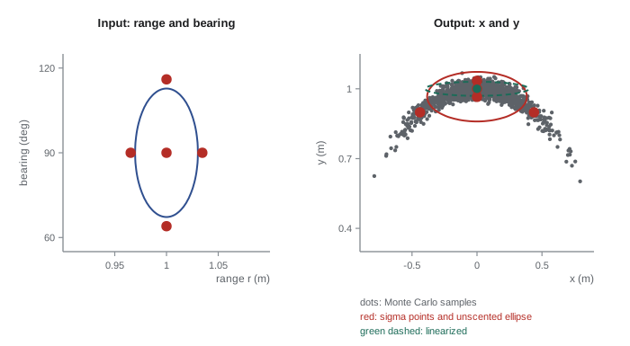
print(f"{name:12s} mean y = {m[1]:.4f} var x = {S[0, 0]:.4f} var y = {S[1, 1]:.5f}")Monte Carlo mean y = 0.9664 var x = 0.0641 var y = 0.00259 linearized mean y = 1.0000 var x = 0.0685 var y = 0.00040 unscented mean y = 0.9663 var x = 0.0640 var y = 0.00494
With 15° of bearing uncertainty, the true mean y is noticeably less than 1 m, because points spread along an arc pull the average inward. The Monte Carlo mean is 0.966 m. Linearization puts the mean at exactly 1 m and reports a variance in y of 0.0004, more than six times too small. The unscented transform matches the Monte Carlo mean to three decimal places using just five function evaluations; its variance in y is about twice the true value, an error on the cautious side, which a filter tolerates far better than the linearized overconfidence. Both get the variance in x, the direction across the bearing, about right. This is the same effect as the banana of lesson 3, and it explains why UKFs often stay consistent in situations where EKFs become overconfident.
Tuning the UKF's parameters matters less than tuning its noise models, but a few rules help. With α near 1 and κ = 3 − n, the sigma points sit about \( \sqrt{3} \) standard deviations from the mean, which suits most robotics problems. Very small α keeps the points close to the mean, which avoids evaluating the model in regions where it is invalid but makes the centre weight large and negative, and can produce a covariance that is not positive definite; square-root implementations of the UKF, which propagate a Cholesky factor directly, avoid this numerical problem.
Choosing among Gaussian and sample-based filters
Three families of filters cover almost all robot state estimation. The table compares them on the properties that usually decide the choice.
| Property | EKF | UKF | Particle filter |
|---|---|---|---|
| Belief representation | One Gaussian | One Gaussian | Weighted samples, any shape |
| Handles nonlinearity by | First-order linearization | Deterministic sigma points | Propagating samples through true models |
| Needs Jacobians | Yes | No | No |
| Multimodal beliefs | No | No | Yes |
| Global localization | No | No | Yes |
| Cost for n states | About n³ | About n³, with 2n + 1 model calls | Grows with particles, which grow quickly with n |
| Typical uses | Drone autopilots, inertial navigation, simple fusion | Strongly nonlinear sensors, attitude estimation | 2-D localization, tracking with clutter, global search |
A practical guide follows from the table. If the system is close to linear over the uncertainty, or Jacobians are available and the uncertainty stays small, the EKF is efficient, well understood and supported by mature libraries. If nonlinearity is significant, Jacobians are tedious or error-prone, or the EKF proves inconsistent, the UKF usually does better at modest extra cost. If the belief can be multimodal, the robot must localize from an unknown start, or measurements include frequent ambiguity, a particle filter is needed, provided the state is low-dimensional enough, which in practice means up to about three to six dimensions. Many real systems combine them: a particle filter for global 2-D localization feeding an EKF or UKF that fuses inertial and wheel data at high rate.
Worked problem
Choosing a filter
For each robot, choose EKF, UKF or particle filter: (a) a warehouse robot that is powered on in an unknown position in a building with many identical aisles; (b) a quadrotor fusing a 1 kHz IMU with a 10 Hz GNSS receiver; (c) a robot fusing a bearing-only camera measurement of a distant landmark with large initial range uncertainty.
Show solution
- (a) The pose is unknown and aisles look alike, so the belief is multimodal: particle filter.
- (b) Errors stay small between GNSS fixes and fast updates matter: an error-state EKF is standard.
- (c) Bearing-only measurements with large range uncertainty are strongly nonlinear: a UKF (or a particle filter for very large uncertainty) handles this better than an EKF.
Answer: (a) Particle filter, (b) EKF, (c) UKF. The decision turns on whether the belief can be multimodal and how large the uncertainty is relative to the curvature of the models.
Common mistakes
MistakeAveraging angular sigma points arithmetically
InsteadUse circular means and wrap angle differences in all covariance sums.
MistakeTreating sigma points as random samples
InsteadThey are deterministic points chosen to match the mean and covariance exactly.
MistakeExpecting a UKF to handle multimodal beliefs
InsteadIt is still a single Gaussian; use a particle filter for multiple hypotheses.
MistakeChoosing α so large that sigma points leave the valid region of the model
InsteadKeep sigma points within regions where the models make sense, especially near singularities.
MistakeForgetting to add process noise in the UKF prediction
InsteadAdd Q to the predicted covariance, or augment the state with the noise.
Summary and key terms
- The UKF approximates the belief with 2n + 1 deterministic sigma points instead of linearizing the model.
- Sigma points are placed at the mean and along columns of a scaled matrix square root of the covariance.
- The transformed mean is accurate to second order, capturing curvature effects the EKF misses.
- The UKF needs no Jacobians and reduces to the Kalman filter for linear systems.
- Angles require circular averaging and wrapped differences in the UKF.
- EKF and UKF are unimodal; particle filters handle multimodal beliefs and global localization.
- Filter choice depends on nonlinearity, possible multimodality, state dimension and computing budget.
- Unscented transform
- A method for propagating a mean and covariance through a nonlinear function using sigma points.
- Sigma points
- Deterministically chosen points that capture a distribution's mean and covariance.
- Unscented Kalman filter
- A Gaussian filter that uses the unscented transform for prediction and update.
- Cholesky factor
- A lower-triangular matrix L with \( \mathbf{L}\mathbf{L}^{\mathsf{T}} = \boldsymbol{\Sigma} \), used as a matrix square root.
- Scaling parameter
- The parameter λ, set by α and κ, that controls sigma point spread.
- Cross-covariance
- The covariance between predicted states and predicted measurements, C.
- State augmentation
- Adding noise variables to the state so that sigma points sample them.
- Circular mean
- An average of angles computed from summed sines and cosines.
- Second-order accuracy
- Matching the true result up to second-order Taylor terms.
- Monte Carlo
- Estimating statistics from many random samples.
Practice problems
Work each problem on paper first, then reveal the answer to check.
How many sigma points for a 3-state pose?
Show answer
7.
With n = 2, α = 1, κ = 1, find λ.
Show answer
\( 1(3) - 2 = 1 \).
Find \( w_0^{(m)} \) for that λ.
Show answer
\( 1/3 \).
Exact mean of \( x^2 \) for \( x \sim \mathcal{N}(2, 1) \)?
Show answer
5.
Linearized mean of \( x^2 \) for the same x?
Show answer
4.
Circular mean of 170° and −170° with equal weights?
Show answer
180°.
What replaces \( \bar{\boldsymbol{\Sigma}}\mathbf{H}^{\mathsf{T}} \) in the UKF gain?
Show answer
The cross-covariance C.
Which filter would you use for global localization?
Show answer
A particle filter.
Why might a UKF stay consistent where an EKF does not?
Show answer
It captures curvature in the mean and covariance.
Name a cost of state augmentation.
Show answer
More sigma points and model evaluations.
Lesson quiz · 5 questions
Score 60% or more to complete this lesson.
Create a free account to save your progress, take quizzes and earn a certificate.