
ROB-310 · Lesson 12 of 12 · 35 min
Capstone: designing and evaluating a localization filter for a mobile robot
This capstone brings the course together in the way estimation work is done in practice. A small indoor delivery robot must know where it is well enough to dock at charging stations and pass through doorways. You will turn that need into numerical requirements, choose sensors and a filter, build a simulation with realistic noise, implement two candidate filters, an extended Kalman filter and a particle filter, and evaluate them with the metrics introduced in earlier lessons: root-mean-square error for accuracy, normalized estimation error squared for consistency, and behaviour under failures. The aim is not only a working filter but evidence that it meets its requirements, which is what a design review, a customer or a safety assessor will ask for.
Requirements
The robot drives at up to 1 m/s around an office floor about 20 m by 15 m. Doorways leave 15 cm of clearance on each side and docking needs the robot within 5 cm and 3° of the dock. Working from these needs, the team writes requirements that can be checked:
| ID | Requirement | How it is verified |
|---|---|---|
| R1 | Position RMSE at most 5 cm and heading RMSE at most 2° in normal operation | Monte Carlo simulation, then motion-capture tests |
| R2 | 95 % of position errors under 10 cm | Error distribution from simulation and tests |
| R3 | Consistent covariance: average NEES within its 95 % chi-square bounds | Monte Carlo NEES test |
| R4 | Update at 50 Hz or faster on the robot computer | Timing on target hardware |
| R5 | Recover from an unknown start or a kidnapping within 30 s of driving | Simulated global-start and kidnapping trials |
| R6 | Survive 10 % outlier measurements without exceeding R2 | Simulation with injected outliers |
Two of these are easy to forget and important. R3 matters because the planner uses the covariance: it slows down and seeks landmarks when uncertainty grows, and it decides whether a doorway is safe to attempt. An overconfident filter defeats that logic. R5 matters because robots are switched on in unknown places, pushed by people and occasionally slip; a filter that can only track from a known start will eventually need a human to rescue it.
Sensors and error budget
The robot has wheel encoders, a MEMS gyro, and a camera that detects coded fiducial markers on walls, giving range and bearing to each visible marker with known identity. Before writing code, an error budget checks that the sensors can plausibly meet the requirements. Between marker sightings, the pose is carried by odometry and the gyro, and its error grows; the markers must be dense enough that the growth between sightings stays inside the budget.
Worked problem
Spacing landmarks from the drift budget
Odometry has a translation error of 2 % of distance travelled (standard deviation) and the gyro-aided heading drifts at a standard deviation of 0.5° per metre. If position error may grow by at most 5 cm (one standard deviation) between marker sightings, how far can the robot drive between sightings?
Show solution
- Along-track error after distance d: \( 0.02d \).
- Lateral error from heading drift grows roughly as \( d \times \sigma_\theta(d)/\sqrt{3} \) for heading error growing linearly from 0; with \( \sigma_\theta = 0.00873d \) rad, lateral error ≈ \( 0.00504d^2 \).
- Along-track limit: \( 0.02d = 0.05 \Rightarrow d = 2.5 \) m.
- Lateral limit: \( 0.00504d^2 = 0.05 \Rightarrow d = 3.15 \) m.
Answer: The along-track error is the binding limit: the robot should see a marker at least every 2.5 m of travel. On a 20 m corridor that means markers about every 2 m on alternating walls, allowing for occlusion by people. The budget turns a vague requirement into a concrete installation rule.
Choosing the filter
The state is the planar pose \( (x, y, \theta) \), three dimensions, which suits both an EKF and a particle filter. The EKF is cheap, smooth and easy to analyse, and with markers every couple of metres the heading uncertainty stays small enough for linearization to work (lesson 6). But an EKF cannot localize globally (R5), and a single wrong marker identification would pull it badly. A particle filter handles R5 naturally and copes better with the occasional outlier, at higher computational cost. A common production answer combines them: a particle filter for global localization and recovery, handing over to an EKF once the particles have converged to a single cluster, with the EKF running at high rate and the particle filter monitoring in the background. This capstone evaluates both filters separately so their strengths can be compared with evidence.
Worked problem
Computational load of the particle filter
The particle filter uses 1,000 particles during tracking and 20,000 during global localization. Each update evaluates up to 4 visible markers per particle, at about 50 floating-point operations per marker likelihood, plus 30 operations per particle for motion sampling. Estimate the operations per update and per second at 50 Hz in both modes.
Show solution
- Per particle: \( 4 \times 50 + 30 = 230 \) operations.
- Tracking: \( 1{,}000 \times 230 = 2.3 \times 10^5 \) per update, \( 1.15 \times 10^7 \) per second.
- Global: \( 20{,}000 \times 230 = 4.6 \times 10^6 \) per update, \( 2.3 \times 10^8 \) per second.
Answer: About 12 million operations per second while tracking and 230 million during global localization, both comfortably within a modern embedded processor running vectorized code. R4 is plausible for both modes, but it must still be confirmed by timing on the target hardware, because memory access and resampling often dominate the arithmetic.
Simulation design
The simulation is the test bench. It drives a ground-truth robot along a route through the office, generates odometry and gyro readings with calibrated noise, and generates marker detections whenever a marker is within 6 m and inside the camera's 90° field of view, with range noise of 3 % of range and bearing noise of 1°. To test R6, a fraction of detections is replaced by outliers with wrong ranges. Each filter runs on the same simulated data. Because a single run can be lucky or unlucky, results are averaged over many Monte Carlo runs with different random seeds, and every run is seeded so that any surprising result can be reproduced and debugged.
Consistency is checked with the average NEES of lesson 5. For a state of dimension n = 3 averaged over M independent runs at one time step, the quantity \( M \times \overline{\text{NEES}} \) follows a chi-square distribution with Mn degrees of freedom, which gives two-sided 95 % bounds on the average. For M = 50 runs, the bounds on the average NEES are about 2.36 and 3.72. If the average falls above the upper bound the filter is overconfident; below the lower bound, underconfident. Time-averaged NEES over a long run is a cruder but common substitute when many runs are impractical.
Worked problem
NEES bounds
For M = 50 runs and n = 3, the chi-square distribution with 150 degrees of freedom has 2.5 % and 97.5 % points of about 117.98 and 185.80. Find the 95 % bounds on the average NEES, and judge a filter whose average NEES is 4.4.
Show solution
- Lower bound: \( 117.98/50 = 2.36 \).
- Upper bound: \( 185.80/50 = 3.72 \).
- 4.4 is above 3.72.
Answer: The bounds are 2.36 to 3.72, and an average of 4.4 means the filter is overconfident: its covariance is too small for its actual errors. The usual remedies are more process noise, larger measurement noise or tempering, and fixing any model mismatch such as an uncalibrated wheel radius.
import numpy as np
rng = np.random.default_rng(2026)
def wrap(a): return (a + np.pi) % (2*np.pi) - np.pi
LM = np.array([[x, y] for x in np.arange(0, 21, 2.0) for y in (-1.0, 9.0)])   # markers every 2 m on two walls
def route(T=600, dt=0.1):                                                   # a loop around the floor
    x = np.array([3.0, 3.0, 0.0]); X, U = [], []
    for k in range(T):
        v, w = 0.8, (0.628 if k % 200 >= 150 else 0.0) + 0.05*np.sin(k*dt)   # 12 m straights, U-turns
        x = np.array([x[0] + v*dt*np.cos(x[2]), x[1] + v*dt*np.sin(x[2]), wrap(x[2] + w*dt)])
        X.append(x); U.append((v*dt, w*dt))
    return np.array(X), np.array(U)
def detect(x):
    out = []
    for j, m in enumerate(LM):
        d = m - x[:2]; r = np.hypot(*d); b = wrap(np.arctan2(d[1], d[0]) - x[2])
        if r < 6 and abs(b) < np.pi/4: out.append((j, r + rng.normal(0, 0.03*r), wrap(b + rng.normal(0, np.radians(1)))))
    return out
def ekf(X, U, Z):
    mu, S = X[0].copy(), np.diag([0.01, 0.01, 0.001]); E, N = [], []
    M = lambda d: np.diag([(0.02*d)**2 + 1e-10, (np.radians(0.5)*d)**2 + 1e-10])
    for k in range(1, len(X)):
        d, dth = U[k]; th = mu[2]
        G = np.array([[1, 0, -d*np.sin(th)], [0, 1, d*np.cos(th)], [0, 0, 1]]); V = np.array([[np.cos(th), 0], [np.sin(th), 0], [0, 1]])
        mu = np.array([mu[0] + d*np.cos(th), mu[1] + d*np.sin(th), wrap(th + dth)]); S = G @ S @ G.T + V @ M(d) @ V.T
        for j, r, b in Z[k]:
            dx, dy = LM[j] - mu[:2]; q = dx*dx + dy*dy; rh = np.sqrt(q)
            H = np.array([[-dx/rh, -dy/rh, 0], [dy/q, -dx/q, -1]]); R = np.diag([(0.03*rh)**2, np.radians(1)**2])
            y = np.array([r - rh, wrap(b - wrap(np.arctan2(dy, dx) - mu[2]))]); Sy = H @ S @ H.T + R
            if y @ np.linalg.solve(Sy, y) > 9.21: continue                   # 99 % gate
            K = S @ H.T @ np.linalg.inv(Sy); mu = mu + K @ y; mu[2] = wrap(mu[2]); S = (np.eye(3) - K @ H) @ S
        e = np.r_[X[k][:2] - mu[:2], wrap(X[k][2] - mu[2])]; E.append(e); N.append(e @ np.linalg.solve(S, e))
    return np.array(E), np.array(N)
res = []
for run in range(30):
    X, U = route(); Un = U + np.c_[rng.normal(0, 0.02*U[:, 0]), rng.normal(0, np.radians(0.5)*U[:, 0])]
    Z = [detect(x) for x in X]
    for k in range(len(Z)):                                                 # 10 % outliers
        Z[k] = [(j, r*rng.uniform(0.3, 0.7) if rng.random() < 0.1 else r, b) for j, r, b in Z[k]]
    E, N = ekf(X, Un, Z); res.append((np.sqrt((E[:, :2]**2).sum(1)), np.degrees(np.abs(E[:, 2])), N))
pos = np.concatenate([r[0] for r in res]); hd = np.concatenate([r[1] for r in res]); nees = np.concatenate([r[2] for r in res])
print(f"EKF position RMSE {np.sqrt(np.mean(pos**2))*100:.1f} cm, 95th percentile {np.percentile(pos, 95)*100:.1f} cm")
print(f"EKF heading RMSE {np.sqrt(np.mean(hd**2)):.2f} deg")
print(f"EKF average NEES {nees.mean():.2f} (consistent filter: about 3)")EKF position RMSE 4.7 cm, 95th percentile 10.3 cm EKF heading RMSE 0.34 deg EKF average NEES 2.51 (consistent filter: about 3)
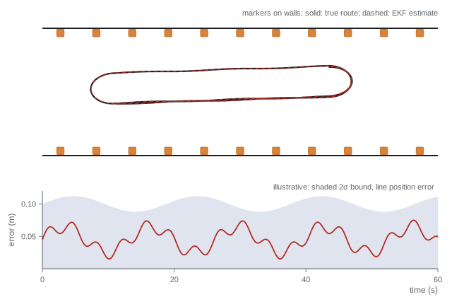
The results are a useful surprise. Heading is excellent, about a third of a degree RMSE, and the 99 % gate keeps the injected outliers from corrupting the estimate. Position, however, only just meets R1 at about 4.7 cm RMSE, and the 95th percentile of about 10.3 cm misses R2's 10 cm limit. Breaking the error down by segment shows it is worst on the long straights, where the markers in view are mostly 4 to 6 m ahead and 3 % range noise means 12 to 18 cm per reading. The simulation has turned a requirement into a design change: add markers at the corridor ends or on pillars so that some are always within 3 m, or choose a camera and marker size with better range accuracy, then re-run the evaluation. Its average NEES of about 2.5 is below the value of 3 expected for a three-dimensional state, so the filter is mildly underconfident: its covariance is somewhat larger than its actual errors. Part of this comes from the start, where the filter is given a 10 cm initial uncertainty although the simulation starts it exactly on the true pose; part comes from linearization at each update. Mild underconfidence is the safe direction, since the planner will be a little more cautious than necessary, but it wastes capability, and the first version of this code was far worse. It added a small floor to the motion noise to avoid zero variances, but the floor on heading was larger than the true heading noise per step, and over a 60 s run it inflated the heading variance severalfold. NEES exposed this immediately, while the RMSE looked fine. The tuning loop of lesson 5 handles the rest: adjust noise models and re-run until the average NEES falls within its bounds, then repeat with logged robot data using NIS and confirm in motion-capture tests.
Evaluating the particle filter and recovery
The particle filter is evaluated on the same runs with 1,000 particles in tracking mode, using the same motion model and a marker likelihood with tempering and a small uniform floor for outliers (lesson 4). Implementing it is left as the main exercise of the capstone, building on the Monte Carlo localization code of lesson 8. In tracking, expect accuracy similar to the EKF but slightly noisier because of sampling, with a NEES that depends on how the covariance is computed from the particles. Its decisive advantage appears in the R5 trials. Started with 20,000 particles spread uniformly over the free space, it should converge to the true pose once the robot has seen a few distinctive marker configurations, and with augmented MCL random injection (lesson 8) it can recover after a simulated kidnapping; measure how many seconds of driving each takes in your layout. The EKF, started at a wrong pose with a small covariance, will not recover: its gate rejects the true markers as outliers, a vivid example of the inconsistency trap described in lesson 6.
Worked problem
Scoring the verification matrix
Suppose the full evaluation, after adding markers and tuning, gives: EKF position RMSE 3 cm, heading RMSE 0.4°, 95th percentile 6 cm, average NEES 2.9 (bounds 2.36 to 3.72 over 50 runs), 4,000 updates per second on target hardware, no global recovery. Particle filter: RMSE 4 cm, 0.6°, 95th percentile 9 cm, NEES 3.1, 300 updates per second at 1,000 particles and 40 per second at 20,000, recovery in 18 s. Which requirements does each meet?
Show solution
- R1 and R2: both meet (3 and 4 cm, under 2°; 95th percentiles 6 and 9 cm under 10 cm).
- R3: both within the NEES bounds.
- R4: EKF easily; particle filter meets 50 Hz in tracking but not during global localization at 40 Hz.
- R5: EKF fails; particle filter meets (18 s under 30 s).
- R6: both met R2 with 10 % outliers in the simulation.
Answer: Neither filter alone meets every requirement: the EKF fails R5, and the particle filter fails R4 during global localization. The combined design, a particle filter for start-up and recovery (accepting a slower update while the robot drives slowly) handing over to an EKF for tracking, meets all six, provided R4 is restated to allow 40 Hz during global localization at reduced speed. Writing that change down, with its justification, is part of the design record.
From simulation to the real robot
Simulation results are necessary but not sufficient. The real robot will show effects the simulation lacked: wheel slip on carpet edges, markers partly hidden by posters, camera exposure changes near windows, timing jitter on the onboard computer. A sound validation plan therefore moves through stages: replaying logged real sensor data through the filters and checking NIS; driving the robot under a motion-capture system or with a total station for ground truth, computing RMSE and NEES on real data; staged failure tests (covering markers, pushing the robot, driving onto a slippery floor); and finally extended operation with monitoring of innovation statistics, rejected-measurement counts and covariance size, logged for later review. Each stage feeds back into the models: the measured odometry error on carpet becomes the motion noise parameters, and the observed marker false-detection rate becomes the outlier probability in the measurement model.
Several lessons from this capstone carry over to any estimation project. Write requirements that can be measured, including consistency and recovery, not just accuracy. Do an error budget before writing code. Compare candidate filters on identical, reproducible data with Monte Carlo statistics rather than single runs. Treat the covariance as a product to be verified, because planners and safety logic depend on it. And plan for failure: gating, monitoring and global recovery are what separate a filter that works in a demonstration from one that runs for months.
Common mistakes
MistakeSpecifying only accuracy requirements
InsteadAlso specify consistency, update rate, robustness to outliers and recovery behaviour.
MistakeJudging a filter from one simulation run
InsteadAverage over many seeded Monte Carlo runs and report distributions.
MistakeTuning on simulated data only
InsteadValidate and retune with logged real data, using NIS where ground truth is missing.
MistakeLetting the gate reject everything after a failure
InsteadMonitor rejection counts and trigger re-initialization or global localization.
MistakeChanging requirements silently when a design falls short
InsteadRecord any requirement change with its justification in the design record.
Summary and key terms
- A localization design starts from measurable requirements for accuracy, consistency, rate, robustness and recovery.
- An error budget relates sensor drift to landmark spacing before any code is written.
- The EKF is efficient and accurate for tracking but cannot localize globally or recover from a bad start.
- The particle filter handles global localization and kidnapping at higher computational cost.
- Monte Carlo simulation with seeded runs provides RMSE, error percentiles and NEES with chi-square bounds.
- A combined particle filter and EKF design often meets requirements that neither meets alone.
- Validation moves from simulation to logged data, ground-truth tests, failure tests and monitored operation.
- Requirement
- A measurable statement of what the system must achieve.
- Error budget
- An allocation of allowable error among sources to check feasibility.
- Root-mean-square error
- The square root of the mean squared estimation error.
- Average NEES
- NEES averaged over runs or time, compared with chi-square bounds to test consistency.
- Chi-square bounds
- Confidence limits on averaged NEES derived from the chi-square distribution.
- Monte Carlo evaluation
- Testing an estimator on many randomized simulated runs.
- Verification matrix
- A table mapping each requirement to its test and result.
- Global localization
- Determining pose from an unknown starting position.
- Ground truth
- An independent, more accurate measurement of the true state used for evaluation.
- Hand-over
- Switching from one estimator, such as a particle filter, to another, such as an EKF.
Practice problems
Work each problem on paper first, then reveal the answer to check.
Odometry error 1 % of distance. Distance for 5 cm error?
Show answer
5 m.
What metric tests consistency in simulation?
Show answer
NEES.
What metric tests consistency on real data?
Show answer
NIS.
Average NEES 2.0 with bounds 2.36 to 3.72. Diagnosis?
Show answer
Underconfident: covariance too large.
Why seed every simulation run?
Show answer
So any result can be reproduced and debugged.
Which requirement does an EKF alone usually fail?
Show answer
Global localization and recovery.
2,000 particles at 200 operations each, 50 Hz. Operations per second?
Show answer
20 million.
Name two real-world effects simulations often miss.
Show answer
Wheel slip on carpet, occluded markers, exposure changes or timing jitter.
What should trigger re-initialization?
Show answer
Many consecutive gated rejections or abnormal innovation statistics.
Why verify the covariance and not just the mean?
Show answer
Planners and safety logic rely on the reported uncertainty.
Lesson quiz · 5 questions
Score 60% or more to complete this lesson.
Create a free account to save your progress, take quizzes and earn a certificate.