
ROB-440 · Lesson 10 of 12 · 28 min
Reliability, maintenance and OEE
A robot cell earns its keep only while it runs. A cell that meets its cycle time on the acceptance test but stops for twenty minutes every few hours for jams, faults and adjustments may produce far less than planned, and the payback calculation of Lesson 11 collapses. This lesson covers how manufacturers measure the effectiveness of automated equipment with overall equipment effectiveness (OEE), how reliability and availability are modelled, what maintenance strategies keep robots running, and how condition monitoring and data analysis catch problems before they stop production. Industrial robots themselves are very reliable, with manufacturers commonly quoting mean times between failures of tens of thousands of hours or more for the arm and controller; in practice, most cell downtime comes from the tooling, sensors, part presentation, upstream and downstream equipment, and programs that do not recover gracefully from abnormal situations.
Overall equipment effectiveness
OEE, popularized by Seiichi Nakajima as part of total productive maintenance (TPM) in Japan in the 1970s and 1980s, measures how much of the planned production time is truly productive. It is the product of three factors. Availability is the share of planned production time during which the equipment actually runs. Performance is the share of the ideal output achieved while running, capturing slow cycles and short stops. Quality is the share of output that is good first time.
Multiplying out the terms shows that OEE also equals the ideal cycle time multiplied by the good count, divided by the planned production time: the share of planned time that would have been needed to make the good parts at the ideal rate. The six big losses of TPM map onto the three factors: breakdowns and set-up or adjustment losses reduce availability; idling and minor stops, and reduced speed, reduce performance; start-up rejects and production rejects reduce quality.
Worked problem
Computing OEE for a robot welding cell
A welding cell is planned to run 450 minutes in a shift. It is stopped for 38 minutes by faults and 22 minutes for a changeover. The ideal cycle time is 52 s. It produces 405 assemblies, of which 391 pass inspection first time. Compute A, P, Q and OEE.
Show solution
- Run time: \( 450 - 38 - 22 = 390 \) minutes, so \( A = 390/450 = 86.7 \) per cent.
- Ideal time for 405 parts: \( 405 \times 52 = 21\,060 \) s \( = 351 \) minutes, so \( P = 351/390 = 90.0 \) per cent.
- Quality: \( Q = 391/405 = 96.5 \) per cent.
- OEE: \( 0.867 \times 0.900 \times 0.965 \approx 75.3 \) per cent.
- Check: \( 391 \times 52 / (450 \times 60) = 20\,332 / 27\,000 = 75.3 \) per cent.
Answer: About 75 per cent; the largest loss is availability, suggesting attention to the faults and to faster changeovers.
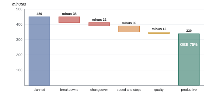
An OEE of 85 per cent is often quoted as world class for discrete manufacturing, a benchmark that dates back to Nakajima's work, though real figures vary widely by industry and many plants run between 40 and 70 per cent. OEE is most useful for tracking one cell or line over time and for directing improvement at the largest losses, not for comparing different kinds of equipment. Because the three factors multiply, a modest weakness in each produces a surprisingly low total: 90 per cent in each gives only 73 per cent overall.
# OEE from a shift log, and a Pareto of downtime causes
log = {"planned_min": 450, "ideal_cycle_s": 52, "total": 405, "good": 391,
       "stops_min": {"gripper part missing": 14, "weld wire jam": 9, "fixture sensor": 6,
                     "upstream starved": 5, "robot collision alarm": 4, "changeover": 22}}
run = log["planned_min"] - sum(log["stops_min"].values())
A = run / log["planned_min"]
P = log["total"] * log["ideal_cycle_s"] / 60 / run
Q = log["good"] / log["total"]
print(f"A={A:.1%}  P={P:.1%}  Q={Q:.1%}  OEE={A*P*Q:.1%}")
total = sum(log["stops_min"].values()); cum = 0
for cause, m in sorted(log["stops_min"].items(), key=lambda kv: -kv[1]):
    cum += m
print(f"{cause:22s} {m:3d} min cumulative {cum/total:5.1%}")A=86.7% P=90.0% Q=96.5% OEE=75.3% changeover 22 min cumulative 36.7% gripper part missing 14 min cumulative 60.0% weld wire jam 9 min cumulative 75.0% fixture sensor 6 min cumulative 85.0% upstream starved 5 min cumulative 93.3% robot collision alarm 4 min cumulative 100.0%
A Pareto chart ranks causes by their contribution, reflecting the common observation that a few causes account for most of the losses. In the example, changeovers and missing parts in the gripper together account for more than half the downtime, which points to two improvement projects: reducing changeover time, perhaps by the single-minute exchange of die (SMED) techniques developed by Shigeo Shingo, and fixing the part presentation that leads to missed grips.
Reliability and availability
Reliability is the probability that a component or system performs its function without failure for a given time. During the useful-life period, when failures occur randomly at a roughly constant rate \( \lambda \), reliability follows the exponential distribution, and the mean time between failures (MTBF) is \( 1/\lambda \). Availability combines how often things fail with how long they take to fix, measured by the mean time to repair (MTTR).
Components in series, where any failure stops the cell, multiply their availabilities, so a cell's availability is lower than that of any of its parts. Redundancy, in which either of two parallel components can do the job, raises availability: the combination fails only when both are down at once.
Worked problem
Availability of a machine tending cell
A cell has a robot with MTBF 40,000 h and MTTR 8 h, a gripper with MTBF 1,500 h and MTTR 0.5 h, a vision system with MTBF 8,000 h and MTTR 2 h, a parts feeder with MTBF 300 h and MTTR 0.25 h, and the CNC machine with MTBF 900 h and MTTR 3 h. What is the cell's inherent availability?
Show solution
- Robot: \( 40\,000/40\,008 \approx 0.99980 \).
- Gripper: \( 1500/1500.5 \approx 0.99967 \).
- Vision: \( 8000/8002 \approx 0.99975 \).
- Feeder: \( 300/300.25 \approx 0.99917 \).
- Machine: \( 900/903 \approx 0.99668 \).
- Product: \( \approx 0.9951 \), or 99.5 per cent.
Answer: About 99.5 per cent from failures alone; the CNC machine and feeder dominate, not the robot. Real availability is lower once minor stops, waiting for maintenance staff and changeovers are included.
This kind of calculation includes only repair time. In practice, a technician must notice the fault, walk to the cell, diagnose it, find a spare part and restart. Mean time to repair as experienced by production is often several times the hands-on repair time, which is why clear fault messages, spare parts stored near the line and operator training to handle simple recoveries have such large effects on availability.
The bathtub curve and failure modes
The failure rate of many products over their lives follows a bathtub curve: a falling rate of early failures caused by manufacturing defects and installation errors, a long period of low and roughly constant random failures, and a rising rate of wear-out failures at the end of life. For robots, early failures appear during commissioning and the first months, which is one reason for run-in periods before acceptance; wear-out affects gearboxes, bearings, cables, seals and batteries. The Weibull distribution, with a shape parameter below 1 for early failures, near 1 for random failures and above 1 for wear-out, is widely used to model these phases.
| Robot cell component | Common failure modes | Typical prevention |
|---|---|---|
| Gearboxes and reducers | Wear, backlash growth, lubricant degradation | Scheduled oil or grease changes; torque and vibration monitoring |
| Cables and dress packs | Conductor breakage, abrasion of hoses | Proper routing, inspection, scheduled replacement |
| Motors and brakes | Brake wear, encoder faults, overheating | Brake tests, temperature monitoring |
| Encoder backup batteries | Loss of position memory when power is off | Replace at intervals specified by the manufacturer |
| Grippers and vacuum cups | Seal leaks, worn fingers, torn cups | Inspection, spare fingers and cups, vacuum monitoring |
| Sensors and cables at fixtures | Misalignment, damage, contamination | Robust mounting, IO-Link diagnostics |
| Software and configuration | Lost or modified programs, corrupted settings | Version-controlled backups, change management |
Maintenance strategies
Reactive maintenance, also called run-to-failure, repairs equipment after it breaks. It is sensible only for inexpensive, non-critical items with quick replacement. Preventive maintenance replaces or services components at fixed intervals of time or usage, following the manufacturer's schedule; robot manuals specify inspection, lubrication, battery replacement and cable checks at intervals such as every few thousand hours. Condition-based maintenance acts when measurements show that a component is deteriorating. Predictive maintenance goes further and forecasts when failure will occur, using trends and models, so that work can be scheduled at a convenient time before it happens. Reliability-centred maintenance (RCM), originally developed in the aviation industry, is a method for choosing the right strategy for each failure mode based on its consequences.
Robot manufacturers offer remote monitoring services that collect data such as motor torques, temperatures, gearbox condition indicators and fault histories, analyse it centrally, and alert users to likely failures. Users can also monitor their own data through OPC UA and MQTT, as Lesson 6 described. Useful indicators include the torque each axis needs for a repeated motion, which rises as gearboxes wear or lubrication fails; the time a vacuum gripper takes to reach its level, which rises as cups wear; the number of retries per hour on a vision pick; and cycle-time drift, which can reveal slow pneumatic actuators or degraded network communication.
Worked problem
Detecting gearbox wear from torque trends
The peak torque of axis 2 during a standard motion averaged 410 N·m with a standard deviation of 6 N·m in its first year. Over the last four weeks the weekly averages were 418, 423, 431 and 437 N·m. Using a control limit three standard deviations above the baseline, should maintenance act?
Show solution
- Upper control limit: \( 410 + 3 \times 6 = 428 \) N·m.
- The last two weekly averages, 431 and 437 N·m, exceed the limit, and the trend has risen steadily by about 6 N·m per week.
- A rising trend in torque for the same motion suggests increasing friction, often from lubricant degradation or gearbox wear.
- Action: inspect, sample or change the lubricant, check for backlash, and plan a gearbox replacement during scheduled downtime if needed.
Answer: Yes; the trend crosses the control limit and is still rising, so maintenance should investigate before it becomes a breakdown.
Spare parts and maintainability
Spare parts strategy balances the cost of holding inventory against the cost of downtime. Critical, long-lead items such as a spare robot motor, a gearbox for the most heavily loaded axis or a spare gripper may be stocked even though they are expensive, because waiting days for delivery could cost far more in lost production. When failures occur randomly, the number of failures in a period follows a Poisson distribution, which allows planners to choose a stock level that covers demand with a chosen probability.
# How many spare grippers to stock? Poisson demand during the resupply lead time
from math import exp, factorial
n_grippers, mtbf_h, hours_per_year = 12, 6000, 6000
lead_time_weeks = 6
failures_per_year = n_grippers * hours_per_year / mtbf_h
mu = failures_per_year * lead_time_weeks / 52           # expected failures during resupply
def p_le(k, mu):
    return sum(exp(-mu) * mu**i / factorial(i) for i in range(k + 1))
print(f"expected failures per year: {failures_per_year:.1f}; during lead time: {mu:.2f}")
for stock in range(0, 5):
print(f"stock {stock}: probability demand covered = {p_le(stock, mu):.3f}")expected failures per year: 12.0; during lead time: 1.38 stock 0: probability demand covered = 0.250 stock 1: probability demand covered = 0.597 stock 2: probability demand covered = 0.837 stock 3: probability demand covered = 0.948 stock 4: probability demand covered = 0.986
Maintainability is designed in. Cells with accessible components, quick-change tooling, clear labelling, standardized parts across cells, good documentation and diagnostic messages that point to the failed component are faster to repair. A computerized maintenance management system (CMMS) schedules preventive tasks, records work orders and failure causes, and tracks spare parts, providing the data needed for MTBF and MTTR analysis. Program and configuration backups belong in the maintenance plan too: a controller failure or an accidental change should be recoverable in minutes from a known good version.
Continuous improvement
Reliability engineering and OEE tracking feed a continuous improvement cycle, often expressed as plan-do-check-act. When a fault recurs, structured root cause analysis, using tools such as the five whys or fishbone diagrams, looks beyond the immediate failure to the underlying cause. A gripper that drops parts might be traced to worn fingers, then to finger material unsuited to an oily part, then to a part change that no one told the integrator about. Fixing the root cause, here by improving engineering change communication, prevents a whole class of future failures. Operators who run the cell every day are often the best source of improvement ideas, which is a central principle of TPM.
Common mistakes
MistakeJudging a cell by its acceptance test cycle time.
InsteadTrack OEE in production and attack the largest losses.
MistakeBlaming the robot for low availability.
InsteadAnalyse all components; tooling, feeders, sensors and machines usually dominate.
MistakeUsing hands-on repair time as MTTR.
InsteadInclude detection, travel, diagnosis and parts retrieval, as production experiences them.
MistakeFollowing only fixed maintenance intervals.
InsteadAdd condition monitoring for key wear items such as gearboxes, cups and cables.
MistakeKeeping no backups of programs and safety configurations.
InsteadVersion and back up programs and settings, and verify safety checksums.
Summary and key terms
- OEE equals availability times performance times quality, or ideal cycle time times good count divided by planned time.
- The six big losses map to availability, performance and quality; Pareto analysis finds the largest causes.
- Availability equals MTBF divided by MTBF plus MTTR; series components multiply availabilities.
- The bathtub curve and Weibull models describe early, random and wear-out failures.
- Maintenance can be reactive, preventive, condition-based or predictive, chosen per failure mode as in RCM.
- Torque trends, vacuum times, retries and cycle-time drift are useful condition indicators for robot cells.
- Spare stocks can be set with Poisson demand; maintainability, CMMS and backups shorten repairs.
- Overall equipment effectiveness (OEE)
- The product of availability, performance and quality.
- Six big losses
- The TPM categories of loss: breakdowns, set-up, minor stops, reduced speed, start-up rejects, production rejects.
- MTBF
- Mean time between failures.
- MTTR
- Mean time to repair.
- Bathtub curve
- A failure-rate profile with early, random and wear-out phases.
- Predictive maintenance
- Maintenance scheduled from forecasts of when failure will occur.
- Reliability-centred maintenance (RCM)
- A method for choosing maintenance strategies by failure consequences.
- SMED
- Single-minute exchange of die, a set of methods for fast changeovers.
- CMMS
- Computerized maintenance management system.
Practice problems
Work each problem on paper first, then reveal the answer to check.
A = 0.9, P = 0.85, Q = 0.98: OEE?
Show answer
About 75 per cent.
Ideal cycle 30 s, 800 good parts, 480 planned minutes: OEE?
Show answer
\( 24\,000/28\,800 \approx 83 \) per cent.
MTBF 500 h, MTTR 2 h: availability?
Show answer
\( 500/502 \approx 99.6 \) per cent.
Two components at 99 per cent each in series: availability?
Show answer
98.0 per cent.
Probability a component with MTBF 2,000 h survives 500 h?
Show answer
\( e^{-0.25} \approx 0.78 \).
What does a Weibull shape parameter above 1 indicate?
Show answer
Wear-out, with failure rate increasing over time.
Name one condition indicator for a vacuum gripper.
Show answer
Time to reach vacuum level, or achieved vacuum.
Why stock a spare gearbox for a critical robot?
Show answer
Long lead times would cause expensive downtime.
Lesson quiz · 5 questions
Score 60% or more to complete this lesson.
Create a free account to save your progress, take quizzes and earn a certificate.