
ROB-440 · Lesson 9 of 12 · 31 min
Warehouse and logistics robots
Warehouses and distribution centres have become one of the fastest-growing markets for robots. Online retail made order profiles smaller and more numerous, customers came to expect next-day or same-day delivery, and labour for repetitive walking and lifting became scarce and expensive in both Canada and the United States. Logistics robots now move pallets and totes, bring shelves and bins to stationary workers, pick individual items, sort parcels, load and unload trucks, and build mixed pallets. ROB-340 covered the localization, mapping and navigation that mobile robots use, ending with a SLAM system for a warehouse robot. This lesson looks at the logistics side: the types of systems, how they are sized, how fleets are managed and integrated with warehouse software, and the safety standards that apply to industrial mobile robots.
The logistics automation landscape
Warehouse operations follow a basic flow: receiving goods from suppliers, putting them away into storage, picking items for customer orders, packing, sorting and shipping. Picking is usually the most labour-intensive step. In a traditional person-to-goods warehouse, pickers walk or drive through aisles with a list, and walking can account for half or more of their time. Automation attacks this in two ways: by moving goods to stationary people, called goods-to-person, or by automating the picking itself.
| System type | What moves | Typical use | Notes |
|---|---|---|---|
| Automated guided vehicle (AGV) | Loads along fixed or virtual paths | Pallet and cart transport in factories and warehouses | Mature; follows wires, tape, magnets or laser reflectors |
| Autonomous mobile robot (AMR) | Loads along paths it plans itself | Tote and cart transport, picking assistance | Navigates by natural features; reroutes around obstacles |
| Goods-to-person shelf robots | Whole shelf units lifted and carried to pick stations | E-commerce fulfilment | Popularized by Kiva Systems, acquired by Amazon in 2012 |
| Cube or grid storage | Robots on top of a grid dig bins out of stacks | Small items in dense storage | Very high storage density |
| Automated storage and retrieval (AS/RS) | Cranes or shuttles in racking | Pallets (unit-load) or totes (mini-load) | High throughput and density; fixed installation |
| Piece-picking robots | Robot arms with vision and suction pick individual items | Each-picking at stations | Grasping mixed items remains challenging; see ROB-400 |
| Autonomous forklifts and tuggers | Pallets and trains of carts | Docks, staging, line feeding | Hybrid of AGV and AMR technology |
| Robotic palletizers and depalletizers | Cases onto or off pallets | Inbound and outbound | Mixed-case palletizing needs stacking algorithms |
AGVs and AMRs
AGVs have been used since the 1950s. Early vehicles followed wires buried in the floor; later ones followed magnetic tape or painted lines, or navigated by laser triangulation from reflectors mounted on walls and columns. They follow defined paths and stop when an obstacle blocks the way. AMRs, which became widespread in the 2010s, localize using natural features of the building with lidar and cameras, plan their own routes on a map, and navigate around obstacles. The distinction has blurred: many modern AGVs use natural-feature navigation, and AMRs in busy facilities are often restricted to defined lanes for predictability. Users choose based on load, path flexibility, traffic and required precision.
| Feature | Traditional AGV | AMR |
|---|---|---|
| Navigation | Wires, tape, magnets or reflectors; fixed paths | Natural features and maps; planned paths |
| Obstacle response | Stops and waits | Replans around if allowed |
| Changing routes | Requires infrastructure or path changes | Software change |
| Typical loads | Heavy pallets and assemblies | Totes, carts, shelves; heavier models exist |
| Predictability | High | Lower unless restricted to lanes |
| Installation | Infrastructure work | Mapping and configuration |
Fleet sizing
The basic question in any mobile robot project is how many vehicles are needed. The answer comes from the number of transport missions per hour and the average time per mission, adjusted for the share of time each vehicle is available, since vehicles charge, wait in traffic and break down.
Worked problem
How many AMRs for line feeding?
AMRs carry kits from a warehouse to an assembly line. There are 48 missions per hour. Each mission involves 140 m of loaded travel and 140 m returning empty at an average 1.0 m/s including slowdowns, 30 s of loading, 30 s of unloading and 20 s of traffic waiting. Vehicles are available 85 per cent of the time after charging, and planners target 80 per cent utilization. How many AMRs are needed?
Show solution
- Travel time: \( 280 / 1.0 = 280 \) s.
- Mission time: \( 280 + 30 + 30 + 20 = 360 \) s.
- Robot-seconds needed per hour: \( 48 \times 360 = 17\,280 \).
- Effective seconds per robot per hour: \( 3600 \times 0.85 \times 0.80 = 2448 \).
- Fleet: \( 17\,280 / 2448 \approx 7.06 \), round up to 8 AMRs.
Answer: Eight AMRs. Because 7.06 is so close to 7, a simulation would show whether 7 can cope with peaks or whether chaining missions to avoid empty return trips could save a vehicle.
# Monte Carlo check of an AMR fleet: queueing of random missions
import numpy as np
rng = np.random.default_rng(440)
def simulate(n_robots, missions_per_hour=48, hours=200):
    t = np.cumsum(rng.exponential(3600 / missions_per_hour, int(missions_per_hour * hours * 1.1)))
    t = t[t < hours * 3600]
    free = np.zeros(n_robots)
    waits = []
    for arrival in t:
        k = np.argmin(free)
        start = max(arrival, free[k])
        waits.append(start - arrival)
        dur = rng.normal(360, 40)                       # mission time, s
        if rng.random() < 0.15:                         # some missions follow a charge or fault
            dur += rng.uniform(300, 900)
        free[k] = start + dur
    w = np.array(waits)
    return w.mean(), np.percentile(w, 95)
for n in (6, 7, 8, 9):
    mean_w, p95 = simulate(n)
print(f"{n} AMRs: mean wait {mean_w:6.0f} s, 95th percentile wait {p95:6.0f} s")6 AMRs: mean wait 2316 s, 95th percentile wait 4984 s 7 AMRs: mean wait 228 s, 95th percentile wait 885 s 8 AMRs: mean wait 52 s, 95th percentile wait 278 s 9 AMRs: mean wait 21 s, 95th percentile wait 145 s
The simulation illustrates a general lesson from queueing theory: as utilization approaches 100 per cent, waiting times grow sharply, and the 95th-percentile wait, which determines whether the assembly line ever starves, grows much faster than the average. Fleet management software vendors typically offer simulation tools for this purpose, and integrators validate them during commissioning.
Goods-to-person and storage systems
Goods-to-person systems bring storage containers to stationary pickers at ergonomic workstations, often with put-to-light displays that show which order container receives each item. Removing walking can raise pick rates from perhaps 60 to 150 lines per hour in manual picking to several hundred lines per hour per station, depending on order profiles. Shelf-lifting robots drive under mobile shelving units and carry them to stations; cube storage systems stack bins in a grid with robots on top that dig out the requested bin; shuttle systems run in each level of a racking structure with lifts at the end of each aisle.
Unit-load AS/RS use cranes running in aisles to store pallets in tall racking, sometimes 30 m or more high, saving floor space and land. A crane's travel time to a storage location depends on horizontal and vertical distance; because the horizontal and vertical drives move simultaneously, the travel time is the larger of the two, the Chebyshev metric.
Worked problem
Single-command cycle time of an AS/RS crane
A pallet crane serves an aisle 90 m long and 24 m high. It travels at 3 m/s horizontally and lifts at 0.8 m/s. Each pick-up or deposit takes 15 s. What is the cycle time to store a pallet at a location 60 m along and 18 m up and return to the input station at the aisle end?
Show solution
- Horizontal time: \( 60/3 = 20 \) s; vertical time: \( 18/0.8 = 22.5 \) s.
- One-way travel: \( \max(20, 22.5) = 22.5 \) s.
- Round trip: \( 45 \) s, plus two handling operations of 15 s each.
- Cycle: \( 45 + 30 = 75 \) s, or 48 single-command cycles per hour.
- Dual-command cycles, storing one pallet and retrieving another in one trip, raise throughput considerably.
Answer: About 75 s, ignoring acceleration; the vertical motion dominates for this location.
# Expected single-command cycle time over random rack locations (Chebyshev travel)
import numpy as np
rng = np.random.default_rng(440)
L, H, vx, vy, t_handle = 90.0, 24.0, 3.0, 0.8, 15.0
x = rng.uniform(0, L, 100_000); y = rng.uniform(0, H, 100_000)
one_way = np.maximum(x / vx, y / vy)
cycle = 2 * one_way + 2 * t_handle
print(f"mean cycle {cycle.mean():.1f} s -> {3600 / cycle.mean():.0f} cycles per hour")
print(f"rack 'shape factor' (time to end / time to top): {(L/vx)/(H/vy):.2f}")mean cycle 70.0 s -> 51 cycles per hour rack 'shape factor' (time to end / time to top): 1.00
Fleet management and integration
A fleet manager assigns missions to vehicles, plans routes, manages traffic at intersections and narrow aisles, schedules charging and handles exceptions such as blocked paths. Task allocation can be as simple as the nearest available robot, or it can optimize across many robots using methods related to the assignment problem. Traffic management prevents deadlocks, in which robots wait for each other in a cycle, often by reserving path segments in advance.
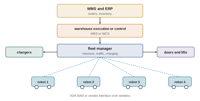
Above the fleet manager sit the warehouse management system (WMS), which manages inventory and orders, and often a warehouse execution system (WES) or warehouse control system (WCS) that orchestrates automation equipment in real time. Mobile robots also interact with building systems: automatic doors, lifts, fire alarm systems that must clear robots from escape routes, and conveyors where they hand over loads.
Mixing fleets from different suppliers has historically meant running several fleet managers that cannot coordinate. VDA 5050, an open interface specification developed by the German automotive industry association VDA together with the mechanical engineering association VDMA, defines how a master control system sends orders to AGVs and AMRs and receives their state, using MQTT and JSON messages. It is increasingly supported by vendors worldwide. The MassRobotics interoperability standard from the United States addresses a related goal of sharing position and status between fleets. Interoperability remains an evolving area in 2026.
Batteries and charging
Mobile robots run on batteries, now mostly lithium-ion chemistries such as lithium iron phosphate, which tolerate frequent partial charging. Charging strategies include opportunity charging during short idle periods, which keeps the fleet working with fewer spare vehicles, and scheduled charging in quiet periods. Battery capacity, charge rate and duty cycle determine the availability figure used in fleet sizing.
Worked problem
Availability from a charging cycle
An AMR draws an average of 400 W while working and has a usable battery capacity of 2.4 kWh. Its charger delivers 1.6 kW. If the robot works until the usable capacity is used and then charges fully, what share of time is it available?
Show solution
- Working time per charge: \( 2.4 / 0.4 = 6 \) h.
- Charging time: \( 2.4 / 1.6 = 1.5 \) h, ignoring the slower final stage of charging.
- Availability: \( 6 / (6 + 1.5) = 80 \) per cent.
- With opportunity charging in idle gaps of a few minutes, much of the charging overlaps time when the robot would be idle anyway, raising effective availability.
Answer: About 80 per cent for full discharge-and-charge cycles; opportunity charging improves this in practice.
Safety standards for industrial mobile robots
Mobile robots raise hazards different from fixed arms: collisions with pedestrians and forklifts, crushing between a vehicle and fixed objects, loads falling from vehicles, and arms mounted on mobile bases, called mobile manipulators. Internationally, ISO 3691-4:2023 covers driverless industrial trucks and their systems, and was under revision at the time of writing. In North America, ANSI/A3 R15.08 addresses industrial mobile robots: Part 1, published in 2020, sets requirements for manufacturers; Part 2, published in 2023, covers integration of IMR systems and applications; and Part 3, for users, was in development. Canada had no national standard specific to industrial mobile robots that we could identify at the time of writing, so Canadian integrators commonly apply ISO 3691-4 and the R15.08 series, along with CSA Z434:26 for robot arms on mobile bases and provincial occupational health and safety requirements. Key design elements include safety-rated laser scanners with protective fields that grow with speed, defined operating zones, speed limits in pedestrian areas, warning lights and sounds, and site risk assessments that consider floor condition, aisle widths and mixed traffic.
Worked problem
Protective field length for a mobile robot
An AMR travels at 1.5 m/s. Its scanner and safety controller respond in 0.10 s, and it decelerates at 1.0 m/s² when its safety brake engages. With a 0.15 m allowance for scanner tolerance and 0.10 m for wheel slip on a dusty floor, how long must the forward protective field be?
Show solution
- Distance during response: \( 1.5 \times 0.10 = 0.15 \) m.
- Braking distance: \( v^2 / (2a) = 2.25 / 2 = 1.125 \) m.
- Allowances: \( 0.15 + 0.10 = 0.25 \) m.
- Field length: \( 0.15 + 1.125 + 0.25 \approx 1.53 \) m ahead of the vehicle.
- At 0.5 m/s the same calculation gives about 0.43 m, which is why fields are switched with speed.
Answer: About 1.5 m at full speed; this assumes a stationary obstacle. Where pedestrians may walk toward the robot, the standards require allowing for their motion too, lengthening the field or lowering speed.
Economics and operations
Warehouse automation projects are judged by throughput, accuracy, labour savings, space savings and flexibility. Highly automated systems such as AS/RS and cube storage give the highest density and throughput but are hard to move or expand. AMR systems can often be added in phases, leased, or offered as robots-as-a-service with monthly fees, which lowers the up-front investment. Peak seasons, such as the period before the end-of-year holidays, matter: a system sized for average demand may fail at the peak, while one sized for the peak sits idle much of the year, which is why many operations combine automation for the base load with temporary labour for peaks. Lesson 11 covers the financial analysis in detail.
Common mistakes
MistakeSizing a fleet from average mission time at 100 per cent utilization.
InsteadInclude availability and a utilization target, then simulate to check waiting at peaks.
MistakeAssuming AMRs need no site preparation.
InsteadCheck floors, Wi-Fi coverage, doors, lifts, aisle widths and mixed traffic.
MistakeTreating mobile robot safety as the vendor's problem alone.
InsteadIntegrators and users must assess the site, zones, speeds and interactions under R15.08 and ISO 3691-4.
MistakeIgnoring empty travel.
InsteadChain missions and position idle robots near demand to cut unloaded trips.
MistakeRunning separate fleets that cannot coordinate.
InsteadPlan interoperability early, using interfaces such as VDA 5050 where supported.
Summary and key terms
- Logistics robots include AGVs, AMRs, goods-to-person systems, AS/RS, piece-picking robots, autonomous forklifts and palletizers.
- AGVs follow defined paths; AMRs navigate by natural features and replan, though the distinction is blurring.
- Fleet size follows from mission rate, mission time, availability and target utilization; simulation captures variability.
- AS/RS cranes move horizontally and vertically together, so travel time is the larger of the two.
- Fleet managers allocate missions, manage traffic and charging, and connect to WMS and WES software, with VDA 5050 aiding interoperability.
- Battery capacity, charging power and opportunity charging determine availability.
- ISO 3691-4 and ANSI/A3 R15.08 are the key mobile robot safety standards; protective fields scale with speed.
- AGV
- Automated guided vehicle, following defined paths.
- AMR
- Autonomous mobile robot, navigating by natural features with planned routes.
- Goods-to-person
- A picking method in which storage units are brought to stationary pickers.
- AS/RS
- Automated storage and retrieval system using cranes or shuttles in racking.
- Fleet manager
- Software that assigns missions to mobile robots and manages traffic and charging.
- WMS
- Warehouse management system, managing inventory and orders.
- VDA 5050
- An open interface for communication between a master control system and AGVs or AMRs.
- Opportunity charging
- Charging batteries during short idle periods.
- Protective field
- The area monitored by a safety scanner in which detection triggers a stop.
Practice problems
Work each problem on paper first, then reveal the answer to check.
60 missions per hour at 300 s each, availability 0.9, utilization 0.8: fleet size?
Show answer
\( 18\,000 / 2592 \approx 6.9 \), so 7 robots.
A crane must move 45 m at 3 m/s and 12 m at 0.6 m/s. One-way time?
Show answer
\( \max(15, 20) = 20 \) s.
Battery 3 kWh, load 0.5 kW, charger 2 kW: availability for full cycles?
Show answer
\( 6/(6 + 1.5) = 80 \) per cent.
Name one difference between an AGV and an AMR.
Show answer
AGVs follow fixed paths and stop at obstacles; AMRs plan paths and can go around them.
What does VDA 5050 standardize?
Show answer
Messages between a master control system and mobile robots, using MQTT and JSON.
Why are scanner protective fields switched with speed?
Show answer
Stopping distance grows with the square of speed, so faster travel needs longer fields.
Which part of R15.08 covers integration?
Show answer
Part 2, published in 2023.
Why do waiting times rise sharply near full utilization?
Show answer
Random arrivals and service times create queues that grow rapidly as spare capacity vanishes.
Lesson quiz · 5 questions
Score 60% or more to complete this lesson.
Create a free account to save your progress, take quizzes and earn a certificate.