
ROB-440 · Lesson 4 of 12 · 28 min
Programming industrial robots
An industrial robot program tells the controller where to move, how fast, with what accuracy, and how to interact with grippers, sensors, PLCs and people. Unlike the research robots of ROB-110, which run ROS 2 nodes on general-purpose computers, most factory robots are programmed in proprietary languages running on the manufacturer's own controller. Each vendor has its own syntax, but the underlying concepts are the same: coordinate frames, tool definitions, motion instructions with speed and blending parameters, input and output signals, program flow and error handling. This lesson teaches those shared concepts, shows short examples in two vendor languages, and covers teaching, offline programming and the calibration that makes offline programs accurate. It does not try to replace vendor training, which every robot programmer eventually needs.
Ways to program a robot
There are four broad methods. Teach pendant programming is the traditional approach: a programmer jogs the robot with a handheld pendant to each position, records it, and writes the program logic on the pendant. It is direct, needs no CAD model, and automatically compensates for robot inaccuracy because each point is a real position. It also takes the robot out of production while programming, and it requires someone to work near the robot, normally in reduced-speed manual mode, which Lesson 8 discusses. Lead-through or hand-guided teaching, common on collaborative robots, lets the programmer move the arm by hand. Offline programming (OLP) creates programs in simulation software from CAD models, then downloads them to the robot; it keeps the robot producing while new programs are written and can generate thousands of points along complex paths. Finally, a growing family of no-code and AI-assisted tools generates motions from task descriptions, demonstrations or vision, though in 2026 these still supplement rather than replace conventional programming in most plants.
| Method | Strengths | Weaknesses | Best for |
|---|---|---|---|
| Teach pendant | No CAD needed; points are exact real positions | Robot out of production; slow for complex paths | Simple pick-and-place, small changes, touch-up |
| Lead-through or hand guiding | Intuitive; fast for simple tasks | Imprecise for exact paths; mostly on cobots | Short-run tasks, small enterprises |
| Offline programming | Robot keeps working; handles complex paths; reusable | Needs accurate models and calibration; software cost | Welding, painting, machining, large projects |
| Task-level and AI-assisted tools | Fast set-up for supported tasks | Limited scope; validation and safety still required | Picking, palletizing patterns, simple assembly |
Coordinate frames
Robot programs describe positions relative to coordinate frames. The world frame is a fixed reference for the cell. The base frame sits at the robot's base. A user frame, called a work object in ABB terminology and a base in KUKA terminology, is attached to a fixture, conveyor or table. The tool frame is attached to the tool, with its origin at the TCP. A position in a program is the pose of the tool frame relative to a chosen user frame. Programming relative to user frames is essential in practice: if a fixture is moved or a second identical fixture is added, only the user frame needs to be re-taught, and every point programmed in it moves along.
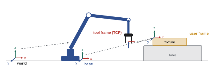
Mathematically, each frame relationship is a homogeneous transformation, as ROB-210 explained. The pose of the tool in the base frame is the product of the transform from base to user frame and the transform from user frame to tool. If the user frame is re-taught after a fixture moves, the first transform changes and all the programmed points follow.
Worked problem
Moving a fixture without re-teaching every point
A fixture's user frame sits at (1,000, 0, 200) mm in the base frame with axes parallel to the base. A program point is (50, 30, 10) mm in the user frame. The fixture is moved and rotated 90° about the vertical axis to a new origin at (600, 700, 200) mm. Where does the point end up in the base frame after only the user frame is re-taught?
Show solution
- Before the move: \( (1000 + 50, 0 + 30, 200 + 10) = (1050, 30, 210) \) mm.
- A 90° rotation about z maps user coordinates \( (x, y) \) to base directions \( (-y, x) \).
- So the point offset becomes \( (-30, 50, 10) \) mm in base directions.
- New position: \( (600 - 30, 700 + 50, 200 + 10) = (570, 750, 210) \) mm.
Answer: (570, 750, 210) mm, achieved by re-teaching three points of the user frame rather than every program position.
A user frame is usually taught with the three-point method: the programmer touches the TCP to the frame origin, a point along the positive x axis, and a point in the xy plane on the positive y side. The controller computes the frame from these points. Accuracy improves if the points are far apart, because an error of 0.2 mm in a point 50 mm from the origin tilts the axis by about 0.23°, while the same error at 500 mm tilts it by only 0.023°.
Defining the tool centre point
The TCP must be defined accurately or reorientations will move the tip off target. The usual teach method is the four-point method: the programmer brings the tool tip to the same fixed reference point, such as a sharp pin, from four or more different orientations. Since the flange poses are known from the robot's joint angles and the tip was at the same location each time, the controller solves for the offset from flange to tip. Additional points or orientations improve the estimate and give an error figure. Automatic TCP calibration stations with light beams measure the tip without human judgement and are common in welding cells, where torch necks bend in minor collisions.
The mathematics is a linear least-squares problem. For each pose \( i \), with flange rotation \( R_i \) and position \( p_i \), the unknown tool offset \( t \) in the flange frame and the unknown fixed point \( c \) satisfy \( R_i t + p_i = c \). Stacking the equations and solving gives both.
# Four-point (here six-point) TCP calibration by least squares
import numpy as np
rng = np.random.default_rng(440)
def rot(ax, ay, az):
    cx, sx, cy, sy, cz, sz = np.cos(ax), np.sin(ax), np.cos(ay), np.sin(ay), np.cos(az), np.sin(az)
    Rx = np.array([[1, 0, 0], [0, cx, -sx], [0, sx, cx]])
    Ry = np.array([[cy, 0, sy], [0, 1, 0], [-sy, 0, cy]])
    Rz = np.array([[cz, -sz, 0], [sz, cz, 0], [0, 0, 1]])
    return Rz @ Ry @ Rx
t_true = np.array([12.0, -4.0, 185.0])        # tool tip in flange frame, mm
c_true = np.array([900.0, 150.0, 300.0])      # fixed reference pin in base frame, mm
A, b = [], []
for k in range(6):
    R = rot(*np.radians(rng.uniform(-35, 35, 3)))
    p = c_true - R @ t_true + rng.normal(0, 0.05, 3)   # flange position with jog error
    A.append(np.hstack([R, -np.eye(3)])); b.append(-p)
x, *_ = np.linalg.lstsq(np.vstack(A), np.hstack(b), rcond=None)
res = np.vstack(A) @ x - np.hstack(b)
print("estimated TCP offset (mm):", np.round(x[:3], 2))
print("estimated pin location (mm):", np.round(x[3:], 2))
print(f"RMS residual: {np.sqrt(np.mean(res**2)):.3f} mm")estimated TCP offset (mm): [ 11.97 -3.93 184.97] estimated pin location (mm): [900. 150.08 299.94] RMS residual: 0.025 mm
Motion instructions
Robot languages provide three basic motion types. A joint move interpolates each joint from start to end angle, coordinated to arrive together; the TCP path is curved and not predictable in Cartesian space, but the move is fast and avoids singularity problems. A linear move drives the TCP along a straight line at controlled speed and orientation; it is required for approaches, insertions, welds and dispensing. A circular move drives the TCP along an arc defined by a via point and an end point. Each instruction also carries a speed, a blending or zone parameter, and the tool and user frame used.
Blending deserves attention because it strongly affects cycle time. An exact stop, called fine in ABB RAPID and FINE in FANUC terminology, makes the robot decelerate fully and settle at the point. A blended point lets the robot round the corner within a zone radius, starting the next motion before reaching the point. Approach and retract points rarely need to be exact, while pick, place and weld start points usually do.
Worked problem
Time saved by blending
A pick-and-place program has eight intermediate via points per cycle, each programmed as an exact stop. Each exact stop costs about 0.12 s of extra deceleration, settling and acceleration compared with a blended corner. The cell runs 1,200 cycles a shift. How much time is saved per shift by blending the via points, and what is the new cycle if the original was 9.5 s?
Show solution
- Saving per cycle: \( 8 \times 0.12 = 0.96 \) s.
- New cycle: \( 9.5 - 0.96 \approx 8.5 \) s, about 10 per cent faster.
- Per shift at the original count: \( 1200 \times 0.96 = 1152 \) s, or about 19 minutes.
- Equivalently, at 8.5 s the same shift time yields about 1,340 cycles instead of 1,200.
Answer: About 1 s per cycle, roughly 19 minutes or 140 extra cycles per shift; the pick and place points themselves stay as exact stops.
Vendor languages
The major robot manufacturers each use their own language. ABB uses RAPID, a structured language with modules, procedures and data declarations. KUKA uses KRL, KUKA Robot Language, with a syntax reminiscent of Pascal. FANUC robots are usually programmed in TP, a line-numbered teach pendant language, with Karel, a Pascal-like language, for advanced logic. Yaskawa Motoman uses INFORM. Universal Robots uses a graphical environment that generates URScript, a Python-like language. Beyond syntax, the concepts transfer: once you understand frames, tool data, motion types, zones and I/O in one language, learning another takes days rather than months.
MODULE PickPlace
  PERS tooldata tGripper := [TRUE, [[0, 0, 185], [1, 0, 0, 0]], [4.5, [0, 15, 110], [1, 0, 0, 0], 0.02, 0.015, 0.012]];
  PERS wobjdata wFixture := [FALSE, TRUE, "", [[1000, 0, 200], [1, 0, 0, 0]], [[0, 0, 0], [1, 0, 0, 0]]];
  CONST robtarget pPick := [[50, 30, 10], [0, 0, 1, 0], [0, 0, 0, 0], [9E9, 9E9, 9E9, 9E9, 9E9, 9E9]];
  PROC main()
    WaitDI diPartReady, 1;                         ! handshake from the PLC
    MoveJ Offs(pPick, 0, 0, 100), v1000, z50, tGripper \WObj:=wFixture;
    MoveL pPick, v200, fine, tGripper \WObj:=wFixture;
    SetDO doGripClose, 1;
    WaitDI diGripClosed, 1 \MaxTime:=2;            ! error handler runs on timeout
    MoveL Offs(pPick, 0, 0, 100), v500, z20, tGripper \WObj:=wFixture;
  ENDPROC
ENDMODULEDEF pick_place()
DECL E6POS approach
BAS(#INITMOV, 0)
$TOOL = TOOL_DATA[1] ; gripper TCP
$BASE = BASE_DATA[2] ; fixture frame
WAIT FOR $IN[10] ; part ready from PLC
approach = XP_PICK
approach.Z = approach.Z + 100
PTP approach C_PTP
LIN XP_PICK ; exact stop at the pick point
$OUT[5] = TRUE ; close gripper
WAIT FOR $IN[11] ; gripper closed
LIN approach C_DIS
ENDLook at the common pattern: wait for a signal that a part is ready, approach above the pick point quickly with blending, move linearly to the exact pick point, close the gripper, confirm with a sensor, and retract. Every industrial pick sequence looks something like this, and every one needs a time-out on the gripper confirmation so that a missed part leads to a defined recovery rather than an endless wait.
Program structure and robustness
Production programs are organized into a main routine that calls procedures for each task, with a home position from which the robot can always start safely. The PLC usually tells the robot which program or job to run through a group of inputs, sometimes called a style or job number, and the robot reports its status back. Lesson 5 describes this handshake from the PLC side. Programs include checks at every step that depends on the outside world: part present, gripper closed, door open, machine ready. A missing confirmation leads to an error routine that moves the robot to a safe position if possible, reports a clear message, and waits for an operator decision.
Recovery after an interruption is the hardest part to get right. If the robot stops in the middle of a path because a guard door opened, the program must resume without colliding, which often means returning along the path or to a known intermediate point. Some integrators write a dedicated home-return routine that analyses where the robot is and picks a safe way back. Variables that track the state of the cell, such as whether the gripper holds a part and which machine is loaded, must survive a power cycle, which is why vendor languages distinguish persistent variables from ordinary ones.
Offline programming and calibration
Offline programs are only as good as the model they come from. A nominal robot model assumes perfect link lengths and joint offsets; a real robot differs by fractions of a millimetre in each link, and the errors accumulate to typical absolute accuracy of perhaps 0.5 to 2 mm across the envelope, even when repeatability is a few hundredths of a millimetre. The cell layout in the simulation also differs from reality. Two kinds of calibration close the gap. Robot calibration identifies the robot's actual kinematic parameters by measuring the TCP at many poses with a laser tracker or similar instrument; manufacturers offer factory-calibrated absolute accuracy options. Cell calibration measures where fixtures, machines and user frames actually are relative to the robot, often by touching reference points with a calibrated TCP. After calibration, offline points typically need only minor touch-up.
| Error source | Typical size before correction | Correction method |
|---|---|---|
| Robot kinematic parameters | 0.5 to 2 mm at the TCP | Robot calibration with a laser tracker; absolute accuracy option |
| TCP definition | 0.1 to 1 mm, more after a collision | Four-point method or automatic TCP measurement |
| User frame and fixture location | Several millimetres in the layout model | Three-point frame teaching; touch-sensing of references |
| Part variation | Depends on the part | Vision, touch sensing or seam tracking at run time |
| Thermal growth of the robot | Up to tenths of a millimetre after warm-up | Warm-up cycles; thermal compensation on some models |
Run-time sensing handles what calibration cannot. Arc welding robots use touch sensing, briefly applying voltage to the wire and touching the part to find its edges, and through-arc seam tracking, which follows a weld joint by measuring current changes as the torch weaves. Vision-guided robots, covered in Lesson 7, locate parts before picking. These methods turn a robot that only repeats taught points into one that adapts to real parts.
ROS 2 and the ROS-Industrial consortium provide drivers for many industrial robots, letting research-style software such as MoveIt plan motions that the vendor controller executes. In production, such systems usually stream or download motions to the vendor controller, which keeps its own safety functions, rather than replacing it. ROB-360 covered the software engineering practices that apply when these systems move from the lab to the factory.
Common mistakes
MistakeProgramming every point in the base frame.
InsteadUse user frames for fixtures and conveyors so that a moved fixture needs only its frame re-taught.
MistakeTeaching a user frame with points close together.
InsteadSpread the three points widely to reduce angular error.
MistakeUsing exact stops everywhere.
InsteadBlend via, approach and retract points; keep exact stops where position matters.
MistakeWaiting for a sensor without a time-out.
InsteadAdd time-outs and error routines that lead to defined recovery.
MistakeExpecting offline programs to run without calibration.
InsteadCalibrate the robot, TCP and cell, then touch up critical points.
Summary and key terms
- Robots are programmed by teach pendant, lead-through, offline programming or task-level tools, often in combination.
- Positions are tool poses relative to user frames; re-teaching a user frame moves all its points.
- The TCP is defined by the four-point method or automatic measurement, a least-squares problem.
- Joint, linear and circular moves carry speed, zone and frame parameters; blending saves cycle time.
- Vendor languages differ in syntax but share concepts: tool data, frames, moves, I/O and error handling.
- Robust programs include handshakes, time-outs, home positions and recovery from interruptions.
- Offline programs need robot and cell calibration; run-time sensing handles part variation.
- Teach pendant
- The handheld device used to jog, program and operate a robot.
- User frame
- A coordinate frame attached to a fixture or workpiece, called a work object or base by some vendors.
- Tool frame
- A frame attached to the tool with its origin at the TCP.
- Four-point method
- Defining the TCP by touching one reference point from several orientations.
- Joint move
- A motion interpolated in joint space, fast but with an unpredictable Cartesian path.
- Linear move
- A motion that drives the TCP along a straight line.
- Zone or blending
- Allowing the robot to round a corner near a point instead of stopping at it.
- Offline programming (OLP)
- Creating robot programs in simulation away from the robot.
- Absolute accuracy
- How closely a robot reaches positions computed from its model.
Practice problems
Work each problem on paper first, then reveal the answer to check.
Why does a taught point compensate for robot inaccuracy?
Show answer
It records the joint angles at the real position, relying only on repeatability.
A user frame at (500, 200, 0) with base-parallel axes holds a point at (20, 10, 5). Base position?
Show answer
(520, 210, 5) mm.
Which motion type is required for a straight weld?
Show answer
A linear move.
Ten via points each cost 0.1 s as exact stops. Saving from blending?
Show answer
1 s per cycle.
Name two vendor robot languages.
Show answer
ABB RAPID, KUKA KRL, FANUC TP or Karel, Yaskawa INFORM, URScript.
Why do robot programs need persistent variables?
Show answer
To remember cell state such as gripper contents through power cycles.
What two calibrations make offline programs accurate?
Show answer
Robot kinematic calibration and cell calibration of frames and fixtures.
What is touch sensing in welding?
Show answer
Using the energized wire to touch the part and find its actual position.
Lesson quiz · 5 questions
Score 60% or more to complete this lesson.
Create a free account to save your progress, take quizzes and earn a certificate.