
STAT-151 · Lesson 1 of 12 · 32 min
Statistics and the scientific method: designing studies
Every measurement a scientist makes is affected by variation. Two seedlings grown in the same tray reach different heights, two readings of the same water sample give slightly different nitrate concentrations, and two patients given the same drug respond differently. Statistics is the discipline that lets scientists draw reliable conclusions in spite of this variation. It tells us how to collect data so that it can answer a question, how to summarize what the data show, and how confident we can be that a pattern is real rather than the product of chance. This course is written for science students working with laboratory and field data. It assumes the calculus of MATH-100 and uses Python, with the numpy and scipy libraries, for every calculation, so that you can rerun and modify each example.
The most important statistical decisions are made before any data are collected. A badly designed study cannot be rescued by clever analysis, while a well-designed one can often be analysed with simple methods. This first lesson therefore covers study design: the difference between observational studies and experiments, the roles of randomization, replication and blocking, the trap of pseudoreplication, blinding, and a first look at how many observations a study needs. Later lessons build the tools to analyse the data that well-designed studies produce.
Populations, samples and variables
A population is the complete set of units a study is about: every trout in a lake, every possible measurement of a reference solution, every adult with high blood pressure in a province or state. A sample is the subset that is actually measured. Because we almost never measure a whole population, we use the sample to estimate population quantities called parameters, such as the population mean, written μ, or a population proportion, written p. Numbers calculated from a sample, such as the sample mean, written x̄, are called statistics. A central theme of this course is that statistics vary from sample to sample, and that this sampling variation can be described and measured.
Each characteristic recorded about a unit is a variable. Variables are either categorical (a species name, a treatment group, whether a seed germinated) or quantitative (a mass, a concentration, a count of insects). Quantitative variables may be continuous, taking any value in a range, or discrete, usually counts. Some categorical variables are ordinal, with a natural order, such as a pain score from 0 to 10 or a disease stage. The type of variable decides which summaries and tests are appropriate, so identifying variables carefully is the first step in planning any analysis.
| Variable | Type | Example from a stream survey |
|---|---|---|
| Site | Categorical (nominal) | Upstream, mid-reach, downstream |
| Water temperature | Quantitative, continuous | 12.4 °C |
| Number of mayfly nymphs per kick sample | Quantitative, discrete (count) | 37 |
| Habitat quality rating | Categorical (ordinal) | Poor, fair, good, excellent |
| Presence of invasive crayfish | Categorical (binary) | Yes or no |
Studies also distinguish explanatory variables, which we think may cause or predict an outcome, from response variables, the outcomes we measure. In a fertilizer trial, the fertilizer dose is explanatory and plant biomass is the response. Naming the response and explanatory variables before collecting data forces a researcher to state the question precisely.
Observational studies and experiments
In an observational study, researchers measure variables without controlling which units receive which conditions. A survey comparing asthma rates in children living near and far from highways is observational: the researchers did not assign families to neighbourhoods. In an experiment, researchers deliberately impose treatments on units and observe the responses. A trial in which seedlings are randomly assigned to receive either a fungicide or water is an experiment.
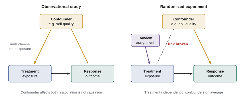
The distinction matters because observational studies are vulnerable to confounding. A confounding variable is related both to the explanatory variable and to the response, so that its effect cannot be separated from the effect being studied. Families living near highways may also have lower incomes, older housing with more mould, and more exposure to tobacco smoke, all of which may influence asthma. An observed association between highway proximity and asthma could be partly or wholly due to these confounders. Observational studies can adjust statistically for confounders that are measured, using methods such as the multiple regression of lesson 11, but they can never rule out confounders that were not measured.
Experiments avoid this problem through random assignment. When treatments are assigned by chance, any characteristic of the units, measured or not, is expected to be balanced between treatment groups. Differences in the response that are larger than chance would produce can then be attributed to the treatment. This is why the randomized controlled trial is regarded as the strongest design for establishing cause and effect in medicine, and why field ecologists go to great lengths to randomize treatments to plots.
Observational studies remain essential. Many questions cannot ethically or practically be answered by experiment: we cannot assign people to smoke, assign lakes to receive acid rain, or assign species to go extinct. Observational designs include cross-sectional studies (a snapshot at one time), cohort studies (following groups forward in time), and case-control studies (comparing people with a disease to people without it, looking back at past exposures). Well-designed observational studies, replicated across many settings and consistent with biological mechanisms, established that smoking causes lung cancer long before any experiment could.
The principles of experimental design
The British statistician Ronald Fisher, working at the Rothamsted agricultural research station in the 1920s, set out three principles that still guide experimental design: randomization, replication and local control, which today we usually call blocking.
Randomization means using a chance mechanism, such as a computer random number generator, to decide which unit gets which treatment. Haphazard assignment by a researcher is not random: people unconsciously put the healthiest-looking plants in the treatment they favour, or fill the first rows of a growth chamber first. Randomization protects against such biases and also provides the logical basis for the statistical tests used later in the course.
import numpy as np
rng = np.random.default_rng(151)

# 24 tomato seedlings, numbered 1-24, to be split into 4 treatments of 6
seedlings = np.arange(1, 25)
treatments = np.repeat(["control", "low N", "medium N", "high N"], 6)
assignment = rng.permutation(treatments)

for t in ["control", "low N", "medium N", "high N"]:
    ids = seedlings[assignment == t]
print(f"{t:9s}: seedlings {', '.join(str(i) for i in ids)}")control : seedlings 12, 13, 14, 15, 20, 23 low N : seedlings 3, 5, 7, 16, 22, 24 medium N : seedlings 1, 4, 8, 9, 17, 18 high N : seedlings 2, 6, 10, 11, 19, 21
The output is one random allocation. Running the code with a different seed would give a different allocation, and that is exactly the point: no person chose which seedling received which treatment. Recording the seed makes the allocation reproducible, so that others can check exactly what was done.
Replication means applying each treatment to several independent units. Replication is what allows us to estimate how much units vary when treated alike, and so to judge whether differences between treatments are larger than that background variation. With one plant per treatment, a difference in growth could be due to the treatment or simply to the particular plants chosen; with ten plants per treatment, we can see how consistent the effect is.
Blocking means grouping units that are similar to one another and randomizing treatments separately within each group. In a field trial, plots near a hedgerow may be shaded and plots near a ditch may be wetter. If every treatment appears once in each region of the field, called a block, differences between regions affect all treatments equally and can be removed in the analysis. Blocking is the experimental counterpart of the advice to compare like with like. Lesson 12 shows how a randomized complete block design is analysed and why it can make an experiment much more sensitive.
import numpy as np
rng = np.random.default_rng(1512)

# Randomized complete block design: 4 fertilizer treatments in each of 5 blocks
treatments = ["A", "B", "C", "D"]
for block in range(1, 6):
    order = rng.permutation(treatments)
print(f"Block {block} (plots left to right): {' '.join(order)}")Block 1 (plots left to right): C D A B Block 2 (plots left to right): B C A D Block 3 (plots left to right): A D B C Block 4 (plots left to right): B D A C Block 5 (plots left to right): A B C D
Each block contains every treatment exactly once, but the order within each block is random. A gradient running across the field from one end of each block to the other therefore cannot systematically favour any treatment.
Experimental units and pseudoreplication
The experimental unit is the smallest unit to which a treatment is independently applied. Identifying it correctly is one of the most important and most frequently mishandled steps in science. Suppose a researcher wants to know whether warming affects plankton growth. She sets the temperature of one aquarium to 15 °C and another to 20 °C, and takes ten water samples from each tank. She has twenty measurements, but only two experimental units: the two tanks. Any difference between the tanks, from a slightly different light level to a contaminated filter, is completely confounded with temperature. Treating the ten samples per tank as independent replicates would be pseudoreplication, a term introduced by the ecologist Stuart Hurlbert in a famous 1984 paper that found the problem in a large fraction of published field experiments.
Pseudoreplication matters because measurements from the same experimental unit tend to be more similar to each other than measurements from different units. Treating them as independent makes the data appear to contain more information than they do, so tests become far too ready to declare effects significant. The cure is to replicate at the level of the experimental unit: several tanks at each temperature, each treated as one observation (for example, by averaging the samples from each tank), or a statistical model that explicitly accounts for the grouping.
import numpy as np
from scipy import stats
rng = np.random.default_rng(15103)

# Simulate a world with NO temperature effect: tanks differ randomly, samples vary within tanks
def one_study(tanks_per_group, samples_per_tank, tank_sd=1.0, sample_sd=0.5):
    groups = []
    for g in range(2):
        tank_means = rng.normal(10, tank_sd, tanks_per_group)
        samples = np.concatenate([rng.normal(m, sample_sd, samples_per_tank) for m in tank_means])
        groups.append((tank_means, samples))
    return groups

reps = 2000
false_pos_pseudo = false_pos_correct = 0
for _ in range(reps):
    (t1, s1), (t2, s2) = one_study(tanks_per_group=1, samples_per_tank=10)
    false_pos_pseudo += stats.ttest_ind(s1, s2).pvalue < 0.05          # samples treated as replicates
    (t1, s1), (t2, s2) = one_study(tanks_per_group=4, samples_per_tank=10)
    m1 = s1.reshape(4, 10).mean(axis=1); m2 = s2.reshape(4, 10).mean(axis=1)
    false_pos_correct += stats.ttest_ind(m1, m2).pvalue < 0.05          # tank means as replicates

print(f"1 tank per group, samples as replicates: false positive rate {false_pos_pseudo/reps:.1%}")
print(f"4 tanks per group, tank means as units: false positive rate {false_pos_correct/reps:.1%}")1 tank per group, samples as replicates: false positive rate 76.2% 4 tanks per group, tank means as units: false positive rate 5.3%
In this simulation there is no temperature effect at all, so a test using the conventional 5 per cent threshold should wrongly declare an effect about 5 per cent of the time. Treating samples from a single tank as replicates gives false positives most of the time, because the test mistakes the random difference between two tanks for a treatment effect. Replicating tanks and analysing tank means restores the correct error rate. The t test used here is explained in lesson 8; for now, notice how the design, not the arithmetic, determines whether the conclusion can be trusted.
Controls, placebos and blinding
A control group receives no treatment, a standard treatment, or a sham treatment, and provides the baseline against which treatments are compared. Without a control, a change after treatment could be due to anything else that changed at the same time: the season, the instrument, or the passage of time itself. In medical research, a placebo, an inactive treatment that looks like the real one, controls for the effect of simply receiving treatment and expecting to improve, which can be substantial for outcomes such as pain.
Blinding prevents knowledge of the treatment from influencing the results. In a single-blind study, participants do not know which treatment they receive. In a double-blind study, neither participants nor the people measuring outcomes know. Blinding is not only for clinical trials. A technician scoring leaf damage, counting cell colonies or reading a histology slide can be unconsciously influenced by knowing which samples were treated; coding samples so the scorer cannot tell them apart is a simple and powerful safeguard.
Worked problem
Spotting design problems
A researcher tests whether a new soil amendment increases wheat yield. She applies it to the eastern half of a field and leaves the western half untreated, then harvests 30 quadrats from each half. The treated half yields 12 per cent more. What are the main design problems, and how could they be fixed?
Show solution
- Experimental unit: the treatment was applied once, to one half of the field, so there is effectively one treated unit and one control unit. The 30 quadrats per half are pseudoreplicates.
- Confounding: any difference between the eastern and western halves, such as soil type, drainage or a previous crop, is confounded with the amendment.
- No randomization: the researcher chose which half received the treatment.
- Fix: divide the field into many plots, group them into blocks of similar plots, and randomly assign the amendment to half the plots in each block. Analyse plot means, with plots as the experimental units.
Answer: The study has only one experimental unit per treatment, no randomization and complete confounding with field position; a randomized block design with many plots would fix all three problems.
How many observations? A first look at sample size
Choosing a sample size is a balance. Too few observations and a real effect may be missed; too many waste money, time and, in animal or human studies, expose more subjects than necessary to procedures or risks. Research ethics boards in both countries, guided by the Tri-Council Policy Statement (TCPS 2) in Canada and the Common Rule in the United States, and animal care committees, expect researchers to justify their sample sizes.
Three quantities drive the required sample size: the size of the effect worth detecting, the amount of variation among units, and how confident we want to be. Lesson 7 develops this properly under the name of power analysis. For now, the key relationship is that the precision of an estimated mean improves with the square root of the sample size. The uncertainty in a sample mean is measured by the standard error, σ/√n, where σ is the standard deviation of individual measurements. Halving the standard error requires four times as many observations.
import numpy as np
sigma = 4.0          # standard deviation of plant height, cm (invented)
for n in (4, 9, 16, 36, 100, 400):
print(f"n = {n:3d}: standard error of the mean = {sigma/np.sqrt(n):.2f} cm")n = 4: standard error of the mean = 2.00 cm n = 9: standard error of the mean = 1.33 cm n = 16: standard error of the mean = 1.00 cm n = 36: standard error of the mean = 0.67 cm n = 100: standard error of the mean = 0.40 cm n = 400: standard error of the mean = 0.20 cm
Going from 4 plants to 16 halves the standard error, but going from 100 to 400 gains only another 0.1 cm. Diminishing returns like these are why careful thought about the effect worth detecting is so valuable: it tells you where to stop.
Sampling in observational and field studies
When we cannot assign treatments, the way units are chosen for measurement becomes critical. A simple random sample gives every unit in the population the same chance of selection, independently of the others. In practice, field scientists often use stratified random sampling, dividing a study area into strata, such as habitat types, and sampling randomly within each, or systematic sampling along transects or grids, which spreads effort evenly. Convenience sampling, measuring whatever is easiest to reach, such as trees near roads or volunteers who answer an advertisement, is prone to bias because the units sampled may differ systematically from the population of interest.
Bias is different from random error. Random error makes estimates scatter around the true value and shrinks as sample size grows. Bias shifts estimates consistently in one direction and does not shrink with more data: a thousand measurements from a miscalibrated thermometer are precisely wrong. Good design aims to remove bias through randomization and calibration, and to control random error through replication and blocking.
Common mistakes
MistakeCorrelation in an observational study shows that one variable causes the other.
InsteadAssociations in observational data may be due to confounding; random assignment in an experiment is the strongest basis for causal claims.
MistakeTaking many measurements from one tank, plot or patient gives many replicates.
InsteadReplicates must be independent experimental units; repeated measurements of one unit are subsamples, and treating them as replicates is pseudoreplication.
MistakeAssigning treatments in a way that seems fair, such as alternating, is as good as randomizing.
InsteadOnly a chance mechanism guarantees that unmeasured factors are balanced on average; haphazard or systematic assignment can introduce bias.
MistakeA larger sample always fixes a biased design.
InsteadMore data reduce random error but not bias; a biased sampling method or uncalibrated instrument stays biased however large the sample.
MistakeBlinding only matters in drug trials.
InsteadAny subjective measurement, from scoring leaf damage to counting colonies, can be influenced by knowing the treatment; coding samples prevents this.
Summary and key terms
- Statistics uses samples to learn about populations while accounting for variation among units and measurements.
- Variables are categorical (nominal, ordinal or binary) or quantitative (continuous or discrete), and their type guides the analysis.
- Observational studies are vulnerable to confounding; random assignment in experiments balances measured and unmeasured factors.
- Fisher’s principles of randomization, replication and blocking underpin sound experimental design.
- The experimental unit is the smallest unit independently assigned a treatment; treating subsamples as replicates is pseudoreplication.
- Controls, placebos and blinding prevent changes over time and expectations from being mistaken for treatment effects.
- The standard error of a mean falls with the square root of sample size, so precision improves with diminishing returns.
- population
- The complete set of units about which a study seeks to draw conclusions.
- sample
- The subset of the population that is actually measured.
- parameter
- A numerical characteristic of a population, such as μ or p.
- statistic
- A number calculated from a sample, used to estimate a parameter.
- confounding variable
- A variable associated with both the explanatory variable and the response, whose effect cannot be separated from the effect studied.
- random assignment
- Using a chance mechanism to decide which unit receives which treatment.
- blocking
- Grouping similar units and randomizing treatments separately within each group.
- experimental unit
- The smallest unit to which a treatment is independently applied.
- pseudoreplication
- Treating non-independent subsamples as if they were independent replicates.
- double-blind
- A design in which neither participants nor those measuring outcomes know which treatment each unit received.
Practice problems
Work each problem on paper first, then reveal the answer to check.
A study finds that students who drink more coffee have higher grades. Is this observational or experimental, and what might confound it?
Show answer
Observational; possible confounders include study habits, time spent studying late, and course load.
Why does random assignment allow causal conclusions?
Show answer
Because it balances all characteristics, measured or unmeasured, between groups on average, so a difference beyond chance can be attributed to the treatment.
A drug is tested on 3 cages of 10 mice each against 3 control cages, with the drug given in the drinking water of each cage. What is the experimental unit?
Show answer
The cage, since the treatment is applied to the whole cage; there are 3 units per group.
Give one way to reduce pseudoreplication in a study with 2 tanks per treatment and 10 samples per tank.
Show answer
Increase the number of tanks per treatment and analyse tank means (or use a model with tank as a grouping factor).
In a field trial, why block by distance from a stream?
Show answer
Soil moisture changes with distance; blocking makes treatment comparisons within similar conditions and removes that variation from the error.
A standard deviation is 6 g. What is the standard error of the mean for n = 9 and n = 36?
Show answer
6/3 = 2 g and 6/6 = 1 g.
How many observations are needed to halve the standard error obtained with n = 25?
Show answer
100, four times as many.
What is the difference between random error and bias?
Show answer
Random error scatters estimates around the true value and shrinks with sample size; bias shifts them consistently and does not shrink.
Why might measuring trees only along a road give a biased estimate of forest health?
Show answer
Roadside trees experience different light, dust, salt and disturbance from interior trees, so they may not represent the forest.
Why should a technician counting bacterial colonies not know which plates were treated?
Show answer
Knowledge of treatment could unconsciously influence borderline counts; blinding removes that bias.
Lesson quiz · 5 questions
Score 60% or more to complete this lesson.
Create a free account to save your progress, take quizzes and earn a certificate.