
STAT-151 · Lesson 7 of 12 · 28 min
Hypothesis tests, power and effect sizes
Confidence intervals answer the question “how big is the effect, and how sure are we?” Hypothesis tests answer a narrower question: “are the data consistent with no effect at all?” Tests are among the most widely used, and most widely misunderstood, tools in science. This lesson sets out the logic of significance testing, explains what a p-value is and is not, introduces the two kinds of error and the power of a test, and shows why effect sizes and confidence intervals should accompany or replace bare statements of significance. It also summarizes the debate about p-values that has reshaped statistical reporting since the American Statistical Association’s 2016 statement.
The logic of a significance test
A significance test begins with a null hypothesis, H₀, usually a statement of no effect or no difference: a new fertilizer does not change mean yield, or the proportion of germinating seeds is the supplier’s stated 0.85. The alternative hypothesis, H₁, states the effect the researcher is looking for. The test asks how surprising the observed data would be if H₀ were true. If they would be very surprising, the data count as evidence against H₀.
The steps are always the same:
1. State H₀ and H₁ in terms of a parameter, before looking at the data.
2. Choose a test statistic that measures how far the data depart from H₀, usually (estimate − null value)/standard error.
3. Find the distribution of the statistic if H₀ is true, the null distribution.
4. Compute the p-value: the probability, under H₀, of a test statistic at least as extreme as the one observed.
5. Interpret the p-value in context, together with an estimate of the effect and its uncertainty.
Worked problem
Does a supplement change chick weight?
Chicks raised on a standard diet reach a mean weight of 250 g at three weeks. An invented sample of 16 chicks on a supplemented diet has mean 262 g and standard deviation 20 g. Is there evidence that the supplement changes mean weight?
Show solution
- H₀: μ = 250 g; H₁: μ ≠ 250 g (two-sided, because a decrease would also matter).
- SE = 20/√16 = 5 g; t = (262 − 250)/5 = 2.40 with 15 degrees of freedom.
- p-value = 2 × P(T₁₅ ≥ 2.40) ≈ 0.030.
- 95 per cent CI: 262 ± 2.131 × 5 = 251.3 to 272.7 g.
Answer: If the supplement had no effect, a sample mean this far from 250 g would occur only about 3 per cent of the time. The data are evidence that the supplement increases weight, by somewhere between about 1 and 23 g; whether a gain that small would matter to a farmer is a separate question.
from scipy import stats
import numpy as np
xbar, s, n, mu0 = 262, 20, 16, 250
se = s/np.sqrt(n)
t = (xbar - mu0)/se
p = 2*stats.t.sf(abs(t), n - 1)
lo, hi = stats.t.interval(0.95, n - 1, loc=xbar, scale=se)
print(f"t = {t:.2f}, df = {n-1}, two-sided p = {p:.4f}")
print(f"95% CI for mu: {lo:.1f} to {hi:.1f} g")t = 2.40, df = 15, two-sided p = 0.0298 95% CI for mu: 251.3 to 272.7 g
What a p-value is, and what it is not
A p-value is a measure of how compatible the data are with the null hypothesis and the assumptions of the test. Small p-values indicate that the data would be unusual if H₀ and the assumptions were true. The American Statistical Association’s 2016 statement on p-values set out six principles, which are worth knowing because the misreadings they correct are extremely common:
| ASA principle (2016) | In plain terms |
|---|---|
| P-values can indicate how incompatible the data are with a specified statistical model. | They measure surprise under H₀ and the test’s assumptions. |
| P-values do not measure the probability that the hypothesis is true, or that the data were produced by chance alone. | p = 0.03 does not mean a 3 per cent chance that H₀ is true. |
| Scientific conclusions should not be based only on whether a p-value passes a threshold. | p = 0.049 and p = 0.051 carry almost identical evidence. |
| Proper inference requires full reporting and transparency. | Selective reporting of significant results distorts the literature. |
| A p-value does not measure the size of an effect or the importance of a result. | Tiny, trivial effects can be highly significant in large samples. |
| By itself, a p-value does not provide a good measure of evidence regarding a model or hypothesis. | Combine it with estimates, intervals and context. |
The second principle connects directly to Bayes’ theorem in lesson 3. The probability that H₀ is true given the data depends on how plausible the hypothesis was before the study, just as the probability of disease after a positive test depends on prevalence. When most hypotheses tested in a field are false, a large share of significant results will be false positives even if each test is performed correctly.
In 2019 a special issue of The American Statistician went further, with an editorial urging researchers to stop using the phrase “statistically significant” altogether. Not all statisticians agree: others argue that a fixed threshold is a useful safeguard against overinterpretation, and some have proposed a stricter default of 0.005 for claims of new discoveries. The common ground is that p-values should be reported exactly (p = 0.03, not p < 0.05), interpreted as a continuous measure of evidence, and never reported without an estimate of the effect and its uncertainty.
Significance levels and the two kinds of error
Many fields still use a significance level α, commonly 0.05, as a decision rule: reject H₀ if p ≤ α. Any such decision can be wrong in two ways.
| H₀ true (no effect) | H₀ false (real effect) | |
|---|---|---|
| Reject H₀ | Type I error (false positive); probability α | Correct; probability = power = 1 − β |
| Do not reject H₀ | Correct; probability 1 − α | Type II error (false negative); probability β |
Lowering α reduces false positives but, for a fixed sample size, increases false negatives. The balance depends on the consequences: in screening a new drug for toxicity, missing a real harm (Type II) may be worse than a false alarm; in claiming a new physical particle, physicists demand the equivalent of α ≈ 3 × 10⁻⁷, the famous “five sigma”, because a false discovery would be so costly.
Failing to reject H₀ is not evidence that H₀ is true. A small or noisy study can easily miss a real effect. “Absence of evidence is not evidence of absence” is a cliché because it is so often forgotten. A confidence interval shows what the data can rule out: an interval of −2 to 25 g for the chick supplement would be consistent with no effect and with a large one.
One-sided and two-sided tests
A two-sided alternative (μ ≠ μ₀) looks for departures in either direction; a one-sided alternative (μ > μ₀) looks in only one. A one-sided test gives half the p-value of a two-sided test when the effect is in the predicted direction, which makes it tempting. It is justified only when an effect in the other direction is impossible or would be treated exactly the same as no effect, and the choice must be made before seeing the data. Most scientific questions call for two-sided tests.
Power and sample size
The power of a test is the probability that it rejects H₀ when a specified real effect exists. Power depends on four things: the size of the true effect, the variability of the data, the sample size and α. Studies with low power are a serious problem in many fields. They often miss real effects, and when they do find significant results, the estimated effects tend to be exaggerated, because only the luckiest overestimates cross the threshold. This exaggeration is sometimes called the winner’s curse.
Researchers should calculate the sample size needed for adequate power, conventionally 80 or 90 per cent, before collecting data. Many funding agencies and ethics boards require this justification. For comparing two means, the power depends on the standardized effect size, introduced below.
import numpy as np
from scipy import stats

def power_two_sample(d, n_per_group, alpha=0.05):
    """Power of a two-sided, two-sample t test for standardized difference d."""
    df = 2*n_per_group - 2
    nc = d*np.sqrt(n_per_group/2)            # noncentrality parameter
    tcrit = stats.t.ppf(1 - alpha/2, df)
    return stats.nct.sf(tcrit, df, nc) + stats.nct.cdf(-tcrit, df, nc)

print("n per group   d = 0.2   d = 0.5   d = 0.8")
for n in (10, 20, 50, 100, 200):
    print(f"{n:11d}   " + "   ".join(f"{power_two_sample(d, n):7.2f}" for d in (0.2, 0.5, 0.8)))

# Smallest n giving 80% power for d = 0.5
n = 2
while power_two_sample(0.5, n) < 0.80:
    n += 1
print(f"n per group for 80% power at d = 0.5: {n}")n per group d = 0.2 d = 0.5 d = 0.8
10 0.07 0.19 0.40
20 0.09 0.34 0.69
50 0.17 0.70 0.98
100 0.29 0.94 1.00
200 0.51 1.00 1.00
n per group for 80% power at d = 0.5: 64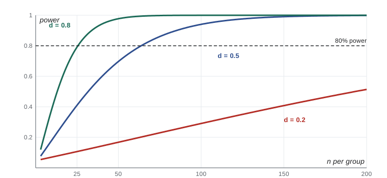
A medium standardized effect of 0.5 needs about 64 subjects per group for 80 per cent power. A small effect of 0.2 needs about 400 per group. Many published laboratory studies use 5 to 10 per group, which gives adequate power only for very large effects.
The simulation below shows the winner’s curse. A real but modest effect is studied many times with small samples; only the significant results are kept, as a biased literature might do.
import numpy as np
from scipy import stats
rng = np.random.default_rng(1517)
true_d, n, reps = 0.3, 15, 20_000
est, sig = [], []
for _ in range(reps):
    a = rng.normal(0, 1, n); b = rng.normal(true_d, 1, n)
    est.append(b.mean() - a.mean())
    sig.append(stats.ttest_ind(b, a).pvalue < 0.05)
est, sig = np.array(est), np.array(sig)
print(f"true effect = {true_d}; power = {sig.mean():.2f}")
print(f"average estimate, all studies:          {est.mean():.2f}")
print(f"average estimate, significant studies: {est[sig].mean():.2f}")true effect = 0.3; power = 0.13 average estimate, all studies: 0.30 average estimate, significant studies: 0.85
Effect sizes
An effect size describes how large an effect is, in units that allow judgement of its importance. The best effect size is usually in the original units: a difference of 12 g in chick weight or 0.3 °C in water temperature, with a confidence interval. When outcomes are measured on different scales, a standardized effect size allows comparison. For two means, Cohen’s d divides the difference by the pooled standard deviation.
Jacob Cohen suggested 0.2, 0.5 and 0.8 as rough benchmarks for small, medium and large effects in behavioural science, but he warned against using them mechanically. Whether an effect matters depends on the subject: a 0.2 standard deviation reduction in blood pressure across a population could prevent many strokes, while a large difference in a trivial outcome may be unimportant. Other common effect sizes are the correlation coefficient r (lesson 10), the proportion of variance explained R² or η² (lessons 10 to 12), and the relative risk and odds ratio for categorical outcomes (lesson 9).
Statistical and practical significance
With very large samples, even trivial effects produce tiny p-values. With small samples, important effects can fail to reach significance. This is why the effect size and interval matter more than the p-value. The example below compares a huge study of a trivial effect with a small study of a large one.
import numpy as np
from scipy import stats
rng = np.random.default_rng(15108)
big_a = rng.normal(100.0, 15, 50_000); big_b = rng.normal(100.4, 15, 50_000)
small_a = rng.normal(100, 15, 8);      small_b = rng.normal(115, 15, 8)

def report(name, a, b):
    sp = np.sqrt(((a.size-1)*a.var(ddof=1) + (b.size-1)*b.var(ddof=1))/(a.size + b.size - 2))
    d = (b.mean() - a.mean())/sp
    p = stats.ttest_ind(b, a).pvalue
    print(f"{name}: difference = {b.mean()-a.mean():5.2f}, d = {d:.2f}, p = {p:.2g}")

report("large study, tiny effect ", big_a, big_b)
report("small study, large effect", small_a, small_b)large study, tiny effect : difference = 0.45, d = 0.03, p = 2.3e-06 small study, large effect: difference = 26.47, d = 1.73, p = 0.0038
The large study detects a difference of less than half a unit on a scale whose SD is 15, a standardized effect of about 0.03, with an extremely small p-value. The small study finds a large effect with a much larger p-value. The small study’s estimate of about 26 is well above the true difference of 15 used in the simulation: with only eight per group, estimates swing widely, which is the winner’s curse again.
Tests and intervals together
A 95 per cent confidence interval and a two-sided test at α = 0.05 are two views of the same calculation: H₀: μ = μ₀ is rejected exactly when μ₀ lies outside the interval. The interval is more informative, because it also shows the range of effect sizes compatible with the data. A good results section reports the estimate, the interval, the exact p-value and the test used, and discusses the practical importance of the effect.
Common mistakes
Mistakep = 0.03 means there is a 3 per cent chance that the null hypothesis is true.
InsteadIt means data this extreme would occur 3 per cent of the time if H₀ and the assumptions were true; the probability of H₀ itself needs prior information.
MistakeA non-significant result shows there is no effect.
InsteadIt shows only that the data cannot rule out no effect; check the confidence interval and the power.
MistakeA smaller p-value means a larger or more important effect.
Insteadp depends on sample size as well as effect size; report the effect and its interval.
MistakeChoose a one-sided test after seeing which way the data point.
InsteadThe direction must be justified and fixed before the data are seen, or the false positive rate doubles.
MistakeA significant result from a small study gives a reliable estimate of the effect.
InsteadSmall significant studies tend to overestimate effects (the winner’s curse).
MistakeReport p < 0.05 or n.s.
InsteadReport exact p-values with effect sizes and confidence intervals.
Summary and key terms
- A significance test asks how surprising the data would be if the null hypothesis and test assumptions were true.
- The p-value is the probability, under H₀, of a result at least as extreme as the one observed; it is not the probability that H₀ is true.
- Type I errors are false positives (probability α); Type II errors are false negatives (probability β); power is 1 − β.
- Power depends on effect size, variability, sample size and α, and should be planned before data collection.
- Low-powered studies miss real effects and exaggerate the effects they do find.
- Effect sizes and confidence intervals convey magnitude and precision, which p-values cannot.
- Report exact p-values, estimates and intervals, and judge practical importance in context.
- null hypothesis
- The hypothesis of no effect or no difference that a test evaluates.
- alternative hypothesis
- The hypothesis describing the effect the researcher seeks evidence for.
- test statistic
- A number summarizing how far the data depart from the null hypothesis.
- p-value
- The probability, if H₀ is true, of a test statistic at least as extreme as that observed.
- significance level
- A threshold α for rejecting H₀, fixed in advance.
- Type I error
- Rejecting a true null hypothesis; a false positive.
- Type II error
- Failing to reject a false null hypothesis; a false negative.
- power
- The probability of rejecting H₀ when a specified alternative is true.
- effect size
- A measure of the magnitude of an effect, in original or standardized units.
- Cohen’s d
- A standardized difference between two means, in pooled standard deviations.
Practice problems
Work each problem on paper first, then reveal the answer to check.
State H₀ and H₁ for testing whether a new catalyst changes mean reaction time from 40 s.
Show answer
H₀: μ = 40 s; H₁: μ ≠ 40 s.
A test gives p = 0.21. What can be concluded?
Show answer
The data are consistent with H₀; an effect has not been demonstrated, but neither has its absence. Check the interval.
For n = 25, x̄ = 52, s = 10, test H₀: μ = 50.
Show answer
t = 1.0, df = 24, two-sided p ≈ 0.33; no evidence of a difference.
What happens to power if the sample size increases?
Show answer
Power increases, because the standard error falls.
What happens to the Type II error rate if α is lowered from 0.05 to 0.01 with n fixed?
Show answer
It increases, so power falls.
Two groups have means 14.0 and 12.5 with pooled SD 3.0. Find Cohen’s d.
Show answer
d = 1.5/3.0 = 0.5, a medium effect by Cohen’s benchmarks.
A 95 per cent CI for a difference is 0.4 to 3.1. Is the two-sided test at α = 0.05 significant?
Show answer
Yes; the interval excludes zero.
Why do significant results from small studies tend to overestimate effects?
Show answer
Only estimates that happen to be large enough cross the significance threshold, so the significant ones are biased upward.
A study of 200,000 people finds p < 0.0001 for a 0.1 mmHg blood-pressure difference. Comment.
Show answer
Statistically significant but almost certainly too small to matter clinically.
When is a one-sided test appropriate?
Show answer
Only when an effect in the other direction is impossible or irrelevant, and the direction is fixed before seeing the data.
Lesson quiz · 5 questions
Score 60% or more to complete this lesson.
Create a free account to save your progress, take quizzes and earn a certificate.