
STAT-151 · Lesson 4 of 12 · 28 min
Probability models for scientific data
Scientific data often follow recognizable patterns. The number of germinated seeds in a tray, the number of plants in a quadrat, the heights of adult men, the waiting time until a radioactive atom decays and the concentration of a contaminant in water each have a typical shape of variation. A probability model, or probability distribution, describes that shape mathematically. Choosing a suitable model lets scientists calculate probabilities, design studies and choose methods of analysis. This lesson introduces random variables and their expected values and variances, then the distributions that appear most often in laboratory and field science: the binomial, Poisson, normal, exponential and lognormal.
Random variables, expected value and variance
A random variable is a numerical outcome of a random process. It is discrete if it takes separate values, usually counts, and continuous if it can take any value in an interval. A discrete random variable is described by its probability mass function, which gives P(X = x) for each value; a continuous one by its probability density function, f(x), whose area over an interval gives the probability of falling in that interval. Probability densities are where the calculus of MATH-100 enters statistics: probabilities are integrals of the density.
The expected value, or mean, of a random variable, written E(X) or μ, is its long-run average. For a discrete variable it is the probability-weighted sum of its values; for a continuous one, the integral of x times the density. The variance, Var(X) or σ², is the expected squared deviation from the mean, and the standard deviation σ is its square root.
Two rules are used constantly. For constants a and b, E(a + bX) = a + bE(X) and Var(a + bX) = b²Var(X). For any random variables, E(X + Y) = E(X) + E(Y), and if X and Y are independent, Var(X + Y) = Var(X) + Var(Y). The second rule, that variances of independent quantities add, is the basis of the propagation of uncertainty in lesson 2 and of the standard error formula.
Worked problem
Expected eggs per nest
In a songbird population, the number of eggs per nest is 3 with probability 0.2, 4 with probability 0.5 and 5 with probability 0.3. Find the mean and standard deviation of clutch size.
Show solution
- E(X) = 3(0.2) + 4(0.5) + 5(0.3) = 0.6 + 2.0 + 1.5 = 4.1 eggs.
- E(X²) = 9(0.2) + 16(0.5) + 25(0.3) = 1.8 + 8.0 + 7.5 = 17.3.
- Var(X) = E(X²) − [E(X)]² = 17.3 − 16.81 = 0.49, so σ = 0.7 eggs.
Answer: The mean clutch is 4.1 eggs with a standard deviation of 0.7 eggs.
The binomial distribution
The binomial distribution describes the number of successes in a fixed number, n, of independent trials, each with the same probability of success, p. It models the number of germinated seeds out of 20, the number of patients responding to a treatment out of 50, or the number of offspring with a recessive trait out of a litter. Its four conditions, sometimes remembered as BINS (binary outcome, independent trials, fixed number n, same probability p), should be checked before it is used.
from scipy import stats

n, p = 20, 0.6          # 20 seeds, germination probability 0.6
X = stats.binom(n, p)
print(f"mean = {X.mean():.1f}, SD = {X.std():.2f}")
print(f"P(exactly 12 germinate) = {X.pmf(12):.4f}")
print(f"P(at most 8 germinate)  = {X.cdf(8):.4f}")
print(f"P(at least 16 germinate) = {X.sf(15):.4f}")mean = 12.0, SD = 2.19 P(exactly 12 germinate) = 0.1797 P(at most 8 germinate) = 0.0565 P(at least 16 germinate) = 0.0510
An important practical point is that the binomial assumes independence and constant p. Seeds from the same parent plant, cells on the same dish or patients treated by the same surgeon may be more alike than the binomial predicts, giving overdispersion: more variation from tray to tray than np(1 − p). When overdispersion is suspected, the trays, dishes or surgeons should be treated as the experimental units, as lesson 1 argued.
The Poisson distribution
The Poisson distribution describes counts of events that occur randomly and independently in time or space at a constant average rate, λ. It models the number of radioactive decays recorded in a minute, the number of bacterial colonies on a plate, the number of plants of a species in a quadrat when individuals are scattered at random, and the number of rare mutations in a stretch of DNA. Its defining feature is that its mean and variance are equal, both λ.
The equality of mean and variance gives ecologists a simple test of spatial pattern. If plants are randomly scattered, counts per quadrat follow a Poisson distribution and the variance-to-mean ratio is about 1. A ratio well above 1 suggests clumping (plants cluster, perhaps around good soil or because seeds fall near the parent), and a ratio below 1 suggests regular spacing (perhaps due to competition). BIOL-208 uses this to study dispersion patterns.
import numpy as np
from scipy import stats
rng = np.random.default_rng(169)

# Invented quadrat counts for two species, 50 quadrats each
random_species = rng.poisson(3.0, 50)
clumped_species = rng.negative_binomial(1.5, 1.5/(1.5 + 3.0), 50)   # same mean, clumped

for name, x in [("random", random_species), ("clumped", clumped_species)]:
    m, v = x.mean(), x.var(ddof=1)
    print(f"{name:8s}: mean {m:.2f}, variance {v:.2f}, variance/mean {v/m:.2f}, "
f"empty quadrats {np.mean(x == 0):.0%} (Poisson predicts {stats.poisson.pmf(0, m):.0%})")random : mean 3.20, variance 3.22, variance/mean 1.01, empty quadrats 2% (Poisson predicts 4%) clumped : mean 2.94, variance 10.42, variance/mean 3.55, empty quadrats 18% (Poisson predicts 5%)
Both species average about three plants per quadrat, but the clumped species has a variance-to-mean ratio well above 1 and many more empty quadrats than the Poisson model predicts. The negative binomial distribution used to simulate it is a standard model for overdispersed counts, such as parasite loads in hosts, where most hosts carry few parasites and a few carry many.
The Poisson distribution is also a good approximation to the binomial when n is large and p is small, with λ = np. Counting rare adverse reactions among many vaccine recipients, for example, is effectively Poisson.
The normal distribution
The normal distribution, with its familiar bell shape, is the most important continuous distribution in statistics. It is specified by its mean μ and standard deviation σ. Many measurements, such as heights, measurement errors in a well-calibrated instrument, and the weights of seeds from a uniform batch, are approximately normal. More importantly, as lesson 5 shows, the sampling distribution of a mean is approximately normal for large samples whatever the shape of the original data, which is why the normal distribution underlies so many statistical methods.
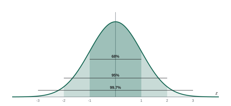
Any normal variable can be converted to the standard normal distribution, with mean 0 and standard deviation 1, by the z-score transformation z = (x − μ)/σ. The 68–95–99.7 rule states that about 68 per cent of values lie within one standard deviation of the mean, 95 per cent within two (more precisely 1.96), and 99.7 per cent within three.
from scipy import stats

# Adult systolic blood pressure treated as normal, mean 122 mmHg, SD 15 mmHg (invented values)
bp = stats.norm(122, 15)
print(f"P(BP > 140)       = {bp.sf(140):.3f}")
print(f"P(110 < BP < 130) = {bp.cdf(130) - bp.cdf(110):.3f}")
print(f"90th percentile   = {bp.ppf(0.90):.1f} mmHg")
print(f"z for 150 mmHg = {(150 - 122)/15:.2f}")P(BP > 140) = 0.115 P(110 < BP < 130) = 0.491 90th percentile = 141.2 mmHg z for 150 mmHg = 1.87
In practice we rarely know whether data are exactly normal, and no real variable is. A normal quantile plot (Q–Q plot), which plots sorted data against the values expected from a normal distribution, is the standard check: approximately normal data fall close to a straight line, while skewness and heavy tails produce curves. Lesson 11 uses the same plot to check regression residuals.
The exponential distribution
The exponential distribution describes the waiting time until an event in a Poisson process: the time between radioactive decays, between arrivals of patients at an emergency department, or until a component fails if failures occur at a constant rate. With rate λ, its mean is 1/λ. It is the continuous partner of the Poisson: if counts in an interval are Poisson, the gaps between events are exponential.
The exponential distribution is memoryless: the probability of waiting at least another t minutes does not depend on how long you have already waited. Radioactive nuclei have no memory of their age, which is why the half-life, the time for half of a sample to decay, is the same however old the sample is. The half-life equals ln 2 / λ, which connects this distribution to the radiometric dating used in BIOL-108 and to drug elimination in pharmacology. STAT-235 treats exponential and related models for reliability and failure times.
Worked problem
Decay of a tracer
Phosphorus-32, used as a tracer in biology laboratories, has a half-life of about 14.3 days. What fraction of an initial sample remains after 30 days, and what is the mean lifetime of a nucleus?
Show solution
- λ = ln 2 / 14.3 = 0.0485 per day.
- Fraction remaining = e^(−0.0485 × 30) = e^(−1.455) ≈ 0.233.
- Mean lifetime = 1/λ ≈ 20.6 days.
Answer: About 23 per cent remains after 30 days; the mean lifetime is about 20.6 days, longer than the half-life because a few nuclei last much longer.
The lognormal distribution
A variable is lognormal if its logarithm is normal. Lognormal distributions arise when many independent factors combine multiplicatively rather than additively, and they are right-skewed and strictly positive. Concentrations of contaminants in water and soil, the sizes of mineral grains, latent periods of infectious diseases, and many biological rates are approximately lognormal. The nitrate data of lesson 2 were simulated this way.
Lognormal data are usually analysed on the log scale, where they are symmetric and the methods for normal data apply. Results are then back-transformed. The back-transformed mean of the logs is the geometric mean, which estimates the median of the lognormal distribution, not its arithmetic mean. Environmental guidelines, such as recreational water quality guidelines for E. coli from Health Canada and the US Environmental Protection Agency, are often written in terms of geometric means of several samples for this reason.
import numpy as np
rng = np.random.default_rng(1514)

# Invented E. coli counts (CFU per 100 mL) from 10 beach samples
counts = np.round(rng.lognormal(mean=np.log(80), sigma=0.9, size=10))
logs = np.log(counts)
print("counts:", counts.astype(int))
print(f"arithmetic mean = {counts.mean():.0f}, median = {np.median(counts):.0f}")
print(f"geometric mean  = {np.exp(logs.mean()):.0f}")
print(f"log-scale mean = {logs.mean():.2f}, log-scale SD = {logs.std(ddof=1):.2f}")counts: [ 59 32 279 171 152 45 361 143 76 47] arithmetic mean = 136, median = 110 geometric mean = 101 log-scale mean = 4.62, log-scale SD = 0.83
The arithmetic mean is pulled up by the largest counts, while the geometric mean sits close to the median. Which to use depends on the question: the arithmetic mean is relevant to total exposure, while the geometric mean describes a typical sample. Guidelines specify which one they mean, and confusing them can make a beach appear to pass or fail when it should not.
Choosing a model
| Situation | Typical model | Key check |
|---|---|---|
| Successes out of a fixed number of independent trials | Binomial(n, p) | Independence; constant p; watch for overdispersion |
| Counts of random events in time or space | Poisson(λ) | Variance about equal to mean |
| Overdispersed counts (clumped organisms, parasites) | Negative binomial | Variance much larger than mean |
| Symmetric continuous measurements; sample means | Normal(μ, σ) | Normal Q–Q plot roughly straight |
| Waiting times with a constant rate | Exponential(λ) | Memoryless; mean equals SD |
| Positive, right-skewed concentrations and sizes | Lognormal | Logs look normal |
A model is a simplification, and the statistician George Box’s remark that all models are wrong but some are useful applies here. The aim is a model close enough to the data that the conclusions drawn from it are reliable, and the checks in the table help decide whether that is so.
Common mistakes
MistakeAny count follows a Poisson distribution.
InsteadThe Poisson requires independent events at a constant rate; clumped or clustered counts are overdispersed and need other models.
MistakeVariances of sums are sums of variances in all cases.
InsteadVar(X + Y) = Var(X) + Var(Y) only when X and Y are independent; correlated quantities need a covariance term.
MistakeA probability density gives the probability of a single value.
InsteadFor continuous variables, probabilities are areas under the density; any single exact value has probability zero.
MistakeThe geometric mean of lognormal data estimates its arithmetic mean.
InsteadIt estimates the median; the arithmetic mean of a lognormal distribution is larger.
MistakeReal data are exactly normal if a test says so.
InsteadNo real variable is exactly normal; check with plots whether normality is a good enough approximation for the method used.
Summary and key terms
- A random variable is a numerical outcome of a random process, described by a mass function (discrete) or density (continuous).
- Expected value is a probability-weighted average; variances of independent variables add.
- The binomial models successes in n independent trials with constant p, with mean np and variance np(1 − p).
- The Poisson models random counts with mean equal to variance; variance-to-mean ratios above 1 indicate clumping.
- The normal distribution follows the 68–95–99.7 rule, and any normal variable can be standardized with z-scores.
- The exponential distribution models waiting times in a Poisson process and is memoryless; half-life = ln 2 / λ.
- Lognormal data are analysed on the log scale, and the geometric mean estimates their median.
- random variable
- A numerical outcome of a random process.
- expected value
- The long-run average value of a random variable.
- binomial distribution
- The distribution of the number of successes in n independent trials with constant success probability.
- Poisson distribution
- A model for counts of independent random events occurring at a constant rate.
- overdispersion
- More variation in counts than a binomial or Poisson model predicts.
- normal distribution
- The symmetric bell-shaped distribution specified by its mean and standard deviation.
- standard normal
- The normal distribution with mean 0 and standard deviation 1.
- exponential distribution
- A model for waiting times between events in a Poisson process.
- lognormal distribution
- A distribution whose logarithm is normal; positive and right-skewed.
- geometric mean
- The exponential of the mean of the logarithms of the data.
Practice problems
Work each problem on paper first, then reveal the answer to check.
A drug cures 70 per cent of patients. In a group of 10, what are the mean and SD of the number cured?
Show answer
Mean = 7, SD = √(10 × 0.7 × 0.3) ≈ 1.45.
Using the binomial formula, find P(all 10 cured).
Show answer
0.7¹⁰ ≈ 0.028.
Colonies on plates average 4 per plate and follow a Poisson distribution. Find P(0 colonies).
Show answer
e⁻⁴ ≈ 0.018.
Quadrat counts have mean 5 and variance 14. What does this suggest?
Show answer
A variance-to-mean ratio of 2.8 suggests clumping (overdispersion).
Heights are normal with mean 170 cm and SD 8 cm. About what percentage are between 154 and 186 cm?
Show answer
About 95 per cent (within 2 SD).
For the same heights, what is the z-score of 182 cm?
Show answer
(182 − 170)/8 = 1.5.
Patients arrive at a clinic at an average rate of 6 per hour. What is the probability of waiting more than 15 minutes for the next arrival?
Show answer
λ = 0.1 per minute; e^(−1.5) ≈ 0.223.
A tracer has λ = 0.1 per day. What is its half-life?
Show answer
ln 2/0.1 ≈ 6.9 days.
Log concentrations have mean 2.0 (natural log). What is the geometric mean concentration?
Show answer
e² ≈ 7.39 units.
If X has SD 3 and Y has SD 4, independent, what is the SD of X + Y?
Show answer
√(9 + 16) = 5.
Lesson quiz · 5 questions
Score 60% or more to complete this lesson.
Create a free account to save your progress, take quizzes and earn a certificate.