
STAT-151 · Lesson 6 of 12 · 29 min
Confidence intervals and the bootstrap
A single number, such as a sample mean of 4.2 mg/L, says nothing about how much it might differ from the truth. Scientific reporting therefore pairs every estimate with a measure of its uncertainty. A confidence interval gives a range of plausible values for a parameter, together with a stated level of confidence. This lesson builds confidence intervals for means and proportions from the sampling distributions of lesson 5, introduces the t distribution that makes them work for small samples, explains what the confidence level does and does not mean, and shows how the bootstrap uses computer resampling to produce intervals when no formula is available.
From a sampling distribution to an interval
Lesson 5 showed that the sample mean is approximately normal with mean μ and standard error σ/√n. About 95 per cent of sample means therefore lie within 1.96 standard errors of μ. Turning the statement around: in about 95 per cent of samples, μ lies within 1.96 standard errors of x̄. So the interval x̄ ± 1.96 σ/√n captures μ in 95 per cent of samples. That is a 95 per cent confidence interval.
Every confidence interval has the same structure: estimate ± critical value × standard error. The product of the critical value and the standard error is the margin of error. Higher confidence requires a larger critical value and so a wider interval; a larger sample shrinks the standard error and narrows the interval.
The t distribution
The formula above requires σ, which is almost never known. Replacing σ with the sample standard deviation s adds uncertainty, particularly in small samples, where s can be well above or below σ by chance. William Sealy Gosset, a chemist at the Guinness brewery in Dublin who published under the pen name Student in 1908, worked out the correct distribution for this situation. If the data are normal, the standardized mean follows a t distribution with n − 1 degrees of freedom.
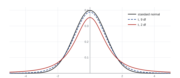
The t distribution is bell-shaped and symmetric like the normal, but with heavier tails that reflect the extra uncertainty from estimating σ. As the degrees of freedom increase, it approaches the standard normal. The table shows how the 95 per cent critical value shrinks towards 1.96.
from scipy import stats
print(" df   t* (95%)   t* (99%)")
for df in (2, 4, 9, 19, 29, 99):
    print(f"{df:3d}   {stats.t.ppf(0.975, df):7.3f}   {stats.t.ppf(0.995, df):7.3f}")
print(f" z {stats.norm.ppf(0.975):7.3f} {stats.norm.ppf(0.995):7.3f}")df t* (95%) t* (99%) 2 4.303 9.925 4 2.776 4.604 9 2.262 3.250 19 2.093 2.861 29 2.045 2.756 99 1.984 2.626 z 1.960 2.576
The one-sample t interval for a mean is therefore:
Worked problem
Mercury in walleye
An invented sample of 12 walleye from a northern lake has mean muscle mercury 0.41 µg/g with standard deviation 0.12 µg/g. Find a 95 per cent confidence interval for the mean mercury concentration of walleye in the lake.
Show solution
- SE = s/√n = 0.12/√12 = 0.0346 µg/g.
- Degrees of freedom = 11; t* = 2.201.
- Margin of error = 2.201 × 0.0346 = 0.076 µg/g.
- Interval: 0.41 ± 0.076 = 0.334 to 0.486 µg/g.
Answer: We are 95 per cent confident that the mean mercury concentration of walleye in the lake is between about 0.33 and 0.49 µg/g. Using z* = 1.96 instead of t* would have produced an interval that is too narrow.
import numpy as np
from scipy import stats
rng = np.random.default_rng(1516)

# Invented mercury data (µg/g) for 12 walleye
hg = np.round(rng.normal(0.41, 0.12, 12), 3)
n, xbar, s = len(hg), hg.mean(), hg.std(ddof=1)
se = s / np.sqrt(n)
lo, hi = stats.t.interval(0.95, n - 1, loc=xbar, scale=se)
print("data:", hg)
print(f"mean = {xbar:.3f}, s = {s:.3f}, SE = {se:.4f}")
print(f"95% t interval: {lo:.3f} to {hi:.3f} µg/g")data: [0.387 0.412 0.399 0.447 0.531 0.599 0.351 0.405 0.433 0.477 0.333 0.605] mean = 0.448, s = 0.089, SE = 0.0257 95% t interval: 0.392 to 0.505 µg/g
This simulated sample of 12 fish, drawn from a population with mean 0.41 and SD 0.12, happens to have a higher mean (0.448) and a smaller SD (0.089) than the summary figures in the worked example, so its interval is a little narrower and sits higher. Different samples from the same lake give different intervals; that variation is exactly what the confidence level accounts for.
What “95 per cent confidence” means
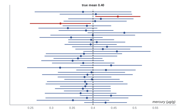
The confidence level describes the method, not any single interval. If we repeated the study many times, drawing new samples and computing a new interval each time, about 95 per cent of the intervals would contain the true mean. Any one interval either contains μ or does not; we just do not know which. It is therefore incorrect, under the frequentist approach used in this course, to say there is a 95 per cent probability that μ lies in a particular interval such as 0.33 to 0.49. The simulation shows the long-run behaviour directly.
import numpy as np
from scipy import stats
rng = np.random.default_rng(15107)
mu, sigma, n, reps = 0.40, 0.12, 12, 10_000
tstar = stats.t.ppf(0.975, n - 1)
covered_t = covered_z = 0
for _ in range(reps):
    x = rng.normal(mu, sigma, n)
    se = x.std(ddof=1) / np.sqrt(n)
    covered_t += abs(x.mean() - mu) <= tstar * se
    covered_z += abs(x.mean() - mu) <= 1.96 * se
print(f"coverage of 95% t intervals (n = 12): {covered_t/reps:.3f}")
print(f"coverage using z* = 1.96 instead: {covered_z/reps:.3f}")coverage of 95% t intervals (n = 12): 0.949 coverage using z* = 1.96 instead: 0.920
The t intervals achieve their promised coverage. Intervals built with 1.96 instead of the t critical value cover the true mean noticeably less often than 95 per cent with only 12 observations, which is why the t distribution matters in the small samples common in laboratory science.
Choosing the sample size
Before collecting data, researchers can choose n to achieve a desired margin of error m. Solving m = z* σ/√n for n gives:
This requires a guess at σ, usually from a pilot study or published work; rounding n up and adding a margin for lost samples is wise. Because n depends on the square of σ/m, halving the margin of error requires four times as many observations, which is often the real constraint on precision in field studies.
Worked problem
Planning a soil survey
A pilot study suggests that soil organic carbon in a region has a standard deviation of about 0.8 per cent. How many cores are needed to estimate the mean within ±0.2 per cent with 95 per cent confidence?
Show solution
- n = (1.96 × 0.8 / 0.2)² = 7.84² ≈ 61.5.
- Round up to 62.
- Allow for perhaps 10 per cent lost or unusable cores: collect about 69.
Answer: Plan for about 70 cores. Halving the margin to ±0.1 per cent would require about 246 usable cores.
Confidence intervals for a proportion
For a proportion, the simplest interval uses the normal approximation: p̂ ± z* √(p̂(1 − p̂)/n), often called the Wald interval. It is easy to compute but performs poorly when n is small or p̂ is near 0 or 1, sometimes giving intervals below 0 or coverage well under 95 per cent. Better alternatives are the Wilson interval and exact (Clopper–Pearson) intervals, which statistical software provides. A quick improvement for hand calculation, the Agresti–Coull method, adds two successes and two failures before computing the Wald interval.
import numpy as np
from scipy import stats

def wald(x, n, conf=0.95):
    z = stats.norm.ppf(0.5 + conf/2); p = x/n
    m = z*np.sqrt(p*(1 - p)/n); return p - m, p + m

def wilson(x, n, conf=0.95):
    z = stats.norm.ppf(0.5 + conf/2); p = x/n
    mid = (p + z**2/(2*n)) / (1 + z**2/n)
    half = z*np.sqrt(p*(1 - p)/n + z**2/(4*n**2)) / (1 + z**2/n)
    return mid - half, mid + half

# 3 infected frogs out of 40 sampled (invented)
x, n = 3, 40
exact = stats.binomtest(x, n).proportion_ci(confidence_level=0.95, method="exact")
print(f"p-hat = {x/n:.3f}")
print("Wald          : %.3f to %.3f" % wald(x, n))
print("Wilson        : %.3f to %.3f" % wilson(x, n))
print("Clopper-Pearson: %.3f to %.3f" % (exact.low, exact.high))p-hat = 0.075 Wald : -0.007 to 0.157 Wilson : 0.026 to 0.199 Clopper-Pearson: 0.016 to 0.204
With 3 positives out of 40, the Wald interval extends below zero, an impossible value for a proportion, while the Wilson and exact intervals stay within sensible bounds and are asymmetric, reflecting the skewness of the sampling distribution when p is small. For any proportion under about 10 per cent or over 90 per cent, or for samples under about 100, report a Wilson or exact interval.
The bootstrap
Formulas exist for intervals around means and proportions, but many scientific quantities, such as a median, a ratio of two means, a correlation, or the dose that kills half the test organisms, have no simple standard error formula. The bootstrap, introduced by Bradley Efron in 1979, solves this with computing power. The idea is to treat the sample as a stand-in for the population and to mimic the sampling process by drawing many resamples of the same size from the data, with replacement. The variation of a statistic across the resamples approximates its sampling distribution.
The percentile bootstrap interval takes the middle 95 per cent of the resampled statistics. More refined versions, such as the bias-corrected and accelerated (BCa) interval, adjust for skewness and bias; scipy.stats.bootstrap computes BCa intervals by default.
import numpy as np
from scipy import stats
rng = np.random.default_rng(1518)

# Invented: times (days) for 15 tagged seeds to germinate; right-skewed
days = np.round(rng.lognormal(np.log(9), 0.5, 15), 1)
print("data:", np.sort(days))
print(f"sample median = {np.median(days):.1f} days")

# Percentile bootstrap by hand
boot = np.array([np.median(rng.choice(days, days.size, replace=True)) for _ in range(10_000)])
lo, hi = np.percentile(boot, [2.5, 97.5])
print(f"percentile bootstrap 95% CI: {lo:.1f} to {hi:.1f} days")

# BCa interval from scipy
res = stats.bootstrap((days,), np.median, n_resamples=10_000, method="BCa", random_state=rng)
print(f"BCa bootstrap 95% CI: {res.confidence_interval.low:.1f} to {res.confidence_interval.high:.1f} days")data: [ 2. 3.7 4.8 5.8 7.1 7.1 7.8 9.2 10.8 11.4 11.9 13.1 15.4 21. 24.5] sample median = 9.2 days percentile bootstrap 95% CI: 5.8 to 11.9 days BCa bootstrap 95% CI: 7.1 to 13.1 days
The bootstrap is not magic. It relies on the sample being representative of the population, so it cannot fix a biased design. It works poorly for very small samples (fewer than about 10 to 15), because a small sample shows only a few possible values. It also needs care for statistics that depend on extremes, such as the maximum, and for dependent data such as time series or clustered measurements, where whole blocks or clusters must be resampled rather than individual values. Within those limits, it is one of the most useful tools in modern data analysis.
Reporting intervals
Good practice is to report the estimate, the interval and the confidence level together, with units and the method if it is not obvious: “mean mercury 0.41 µg/g (95 per cent CI 0.33 to 0.49, t interval, n = 12)”. Graphs should state whether error bars show standard deviations, standard errors or confidence intervals, because the three differ greatly in width and meaning. A standard deviation describes the spread of the data; a standard error is roughly a 68 per cent interval for the mean; a 95 per cent confidence interval is about twice as wide as a standard error bar for moderate n.
| Error bar | What it describes | Width for n = 10 (s = 1) |
|---|---|---|
| Standard deviation | Spread of individual observations | ±1.00 |
| Standard error | Precision of the mean (about 68% confidence) | ±0.32 |
| 95% confidence interval | Plausible range for the mean | ±0.72 |
Common mistakes
MistakeThere is a 95 per cent probability that the true mean lies in this particular interval.
InsteadThe 95 per cent describes the long-run success rate of the method; a specific interval either contains the mean or does not.
MistakeA 95 per cent confidence interval contains 95 per cent of the data.
InsteadIt is a range for the parameter (such as the mean), not for individual observations, and is usually much narrower than the data.
MistakeUse z* = 1.96 for any sample size.
InsteadWhen σ is estimated from a small sample, use the t critical value with n − 1 degrees of freedom.
MistakeThe Wald interval works for any proportion.
InsteadIt performs badly for small samples or proportions near 0 or 1; use Wilson or exact intervals.
MistakeThe bootstrap creates new information from the data.
InsteadIt only approximates the sampling distribution; it cannot overcome a small or biased sample.
MistakeError bars on a graph need no explanation.
InsteadAlways state whether bars show SD, SE or a confidence interval, because they differ greatly in width.
Summary and key terms
- A confidence interval has the form estimate ± critical value × standard error.
- The t distribution, with n − 1 degrees of freedom, replaces the normal when σ is estimated from the data.
- The confidence level is the long-run proportion of intervals that capture the parameter, not the probability for one interval.
- Higher confidence widens intervals; larger samples narrow them, but only in proportion to √n.
- For proportions, Wilson and exact intervals are preferable to the simple Wald interval when n is small or p̂ is extreme.
- The bootstrap resamples the data with replacement to approximate the sampling distribution of almost any statistic.
- Report estimates with intervals, units, confidence level and method, and label error bars clearly.
- confidence interval
- A range of plausible values for a parameter produced by a method with a stated long-run success rate.
- confidence level
- The proportion of intervals, over repeated samples, that would contain the parameter.
- margin of error
- The critical value times the standard error; half the width of a symmetric interval.
- t distribution
- A symmetric, heavy-tailed distribution used for inference about means when σ is estimated.
- degrees of freedom
- The number of independent pieces of information available to estimate variability; n − 1 for a one-sample t.
- critical value
- The multiplier, such as t* or z*, that sets the confidence level.
- Wilson interval
- A score-based confidence interval for a proportion with good coverage for small n.
- bootstrap
- A resampling method that draws repeated samples with replacement from the data to estimate a sampling distribution.
- resample
- A sample of the same size drawn with replacement from the observed data.
- percentile interval
- A bootstrap interval formed from the middle percentage of resampled statistics.
Practice problems
Work each problem on paper first, then reveal the answer to check.
A sample of 25 has x̄ = 18.0 and s = 5.0. Find a 95 per cent CI for μ (t* = 2.064).
Show answer
SE = 1.0; 18.0 ± 2.06, or 15.9 to 20.1.
How does the interval change if the confidence level rises to 99 per cent?
Show answer
It becomes wider, because the critical value increases.
What sample size gives a margin of ±1 with 95 per cent confidence if σ ≈ 6?
Show answer
n = (1.96 × 6)² = 138.3, so 139.
Why is the t distribution used instead of the normal for small samples?
Show answer
Because σ is estimated by s, which adds uncertainty; the t distribution’s heavier tails account for it.
A study reports a 95 per cent CI of 2.1 to 3.4. A student says 95 per cent of the measurements lie in that range. Correct this.
Show answer
The interval is for the population mean, not for individual measurements.
In 200 water samples, 46 contain a contaminant. Compute the Wald 95 per cent interval.
Show answer
p̂ = 0.23; SE ≈ 0.0298; 0.23 ± 0.058, or 0.172 to 0.288.
Why might the Wald interval be unsuitable for 1 positive in 25 tests?
Show answer
n is small and p̂ is near 0, so the normal approximation fails and the interval may go below zero.
Describe how to obtain a percentile bootstrap interval for a median.
Show answer
Resample the data with replacement many times, compute the median each time, and take the 2.5th and 97.5th percentiles.
Give one situation in which the bootstrap performs poorly.
Show answer
Very small samples, statistics based on extremes, or dependent data resampled as if independent.
A figure shows means with error bars but no legend for them. What should be added?
Show answer
A statement of whether the bars are SD, SE or confidence intervals, with n.
Lesson quiz · 5 questions
Score 60% or more to complete this lesson.
Create a free account to save your progress, take quizzes and earn a certificate.