
CON-250 · Lesson 11 of 12 · 35 min
Equipment productivity and cost
An earthwork estimate rests on two numbers for every machine: how much it produces per hour, and how much it costs per hour. Divide one into the other and you have a unit cost per cubic meter or cubic yard. Get either number wrong and the estimate, the schedule and possibly the profit on the job go with it. This lesson shows how to estimate production from cycle times, how to balance a loader with its trucks, how to calculate owning and operating costs, and how to turn them into unit costs and decisions about renting or owning.
The production equation
Almost all earthmoving equipment works in cycles: load, travel, dump, return. Production per hour is the load per cycle multiplied by the number of cycles per hour, reduced by a job efficiency factor that accounts for the time a machine is not actually producing.
- Load per cycle is the volume actually carried, usually in loose volume, and later converted to bank volume for the estimate. For buckets, it equals the rated heaped capacity times a fill factor that depends on the material: perhaps 0.95 to 1.0 for loose sand and gravel, 0.8 to 0.9 for common earth and 0.6 to 0.75 for blasted rock.
- Cycle time is the total time for one complete cycle, from start of loading to start of the next loading.
- Job efficiency E accounts for delays, operator breaks, waiting, minor maintenance, moving and supervision. A common assumption is a 50-minute working hour, or E = 0.83; poor conditions may justify 0.67 (40 minutes) and excellent conditions 0.92 (55 minutes).
Manufacturers publish performance handbooks with cycle times, fill factors and production curves for their machines. Contractors build their own records from past jobs, which are more reliable than handbook values because they reflect the contractor's operators, conditions and management.
Excavator and loader production
For an excavator loading trucks, the cycle is dig, swing loaded, dump and swing back. A mid-size excavator in common earth typically cycles in 15 to 25 seconds. Swing angle, digging depth, the hardness of the material and the operator's skill all affect it. Loading over 90 degrees takes longer than loading over 45 degrees, and trucks positioned badly can add several seconds to every cycle.
Worked problem
Excavator production
An excavator with a 2.5 cu yd heaped bucket loads common earth (fill factor 0.90, swell 25 percent) with a 20-second cycle. Job efficiency is a 50-minute hour. What is its production in bank cubic yards per hour?
Show solution
- Load per cycle = 2.5 × 0.90 = 2.25 LCY.
- Cycles per hour = 3,600 ÷ 20 = 180.
- Production = 2.25 × 180 × 50/60 = 337.5 LCY per hour.
- Bank production = 337.5 ÷ 1.25 = 270 BCY per hour.
Answer: About 270 BCY per hour.
That figure is the excavator's potential. It is only achieved if trucks are always waiting to be loaded. If trucks are late, the excavator waits, and its real production falls. That is why the loader and trucks must be considered together.
Haul unit cycle time
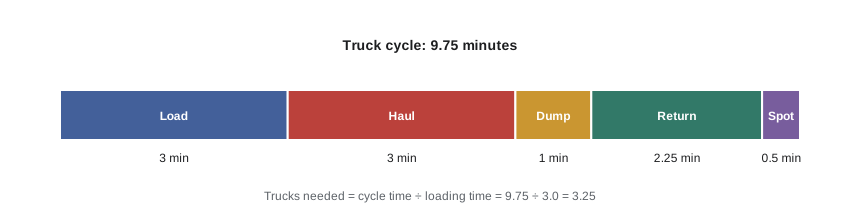
A truck's cycle has five parts: loading, hauling loaded, dumping and turning, returning empty, and spotting and waiting at the loader.
- Loading time is the number of bucket passes needed to fill the truck times the loader's cycle time. Matching truck size to bucket size so that the truck is filled in a whole number of passes, typically 3 to 6 for wheel loaders and 4 to 8 for excavators, avoids partial passes.
- Haul and return times are the distances divided by the average speeds. Speeds come from rimpull charts at the effective grade of each section, reduced for acceleration, deceleration and speed limits on the site.
- Dump and turn time is typically 0.5 to 1.5 minutes depending on the dumping area and spreading method.
- Spot and wait time covers maneuvering under the loader and any queueing.
Worked problem
Truck cycle time
Trucks are loaded to about 20 LCY by the excavator above (2.25 LCY per pass, 20-second cycle). The haul is 0.75 mile at an average loaded speed of 15 mph; the return at 20 mph. Dump and turn takes 1.0 minute and spot and wait 0.5 minute. Find the truck cycle time.
Show solution
- Passes = 20 ÷ 2.25 = 8.9, so 9 passes; loading = 9 × 20 s = 180 s = 3.0 min.
- Haul = 0.75 mile ÷ 15 mph × 60 = 3.0 min.
- Return = 0.75 ÷ 20 × 60 = 2.25 min.
- Cycle = 3.0 + 3.0 + 1.0 + 2.25 + 0.5 = 9.75 min.
Answer: 9.75 minutes per cycle.
Balancing the fleet
The number of trucks needed to keep the loader busy equals the truck cycle time divided by the time it takes to load one truck. If the answer is a fraction, the choice is between rounding down, so the trucks are always busy but the loader sometimes waits, or rounding up, so the loader is always busy but trucks sometimes queue. The cheaper option depends on the relative costs of the loader and the trucks.
Worked problem
How many trucks?
Using the cycle above, how many trucks are needed, and what is the hourly production with 3 trucks and with 4 trucks (50-minute hour)?
Show solution
- N = 9.75 ÷ 3.0 = 3.25 trucks.
- With 3 trucks, the trucks limit production: 3 × 20 × (60 ÷ 9.75) × 0.833 = 308 LCY/h.
- With 4 trucks, the excavator limits production: it loads one truck every 3.0 min, so 20 × 20 × 0.833 = 333 LCY/h.
- The fourth truck adds about 25 LCY/h (8 percent) but adds a whole truck's cost; compare cost per cubic yard for both options.
Answer: 3.25 trucks needed; 308 LCY/h with 3 trucks, 333 LCY/h with 4.
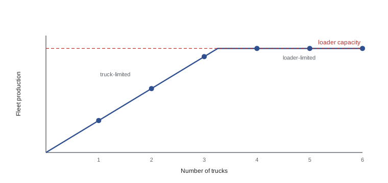
In practice, trucks bunch up, haul roads change and loaders slow down, so actual production is a little below the simple calculation. Experienced estimators allow for this by using a slightly lower efficiency or by simulation. On site, the superintendent watches for trucks queuing at the loader (too many trucks) or the loader sitting idle (too few), and adjusts the fleet daily.
Dozer and scraper production
Dozer production is usually read from manufacturer curves that give the maximum production for each blade against the push distance, then corrected by factors for operator skill, material, slot or side-by-side dozing, grade, visibility, job efficiency and blade type. Dozing downhill increases production by roughly 2 percent per 1 percent of grade; uphill reduces it.
Scraper production follows the same cycle method as trucks: load time (with or without a push dozer), haul time, spread time and return time. One push dozer can serve several scrapers if the scraper cycle is long compared with the push time, and the number of scrapers per pusher is balanced in the same way as trucks per loader.
Owning costs
An equipment hour costs money whether or not the machine is working. Owning costs are those that arise from owning the machine, independent of how hard it is used.
- Depreciation: the loss of value over the machine's economic life. The simplest method is straight-line: purchase price less salvage value, divided by the total hours of the economic life. Tires are often excluded from the purchase price and treated as an operating cost.
- Interest, insurance, taxes and storage: often estimated as a percentage of the average annual investment, the average value of the machine over its life.
Here P is the purchase price, S the salvage value and n the life in years. The average annual investment formula reflects the fact that the money tied up in a machine falls as it depreciates.
Operating costs
Operating costs arise only when the machine works, and they are roughly proportional to hours of use.
- Fuel: diesel consumption depends on the engine and the load factor. A mid-size excavator might burn 5 to 9 gallons per hour in typical work.
- Lubricants, filters and fluids, often estimated as a percentage of fuel cost or from manufacturer data.
- Tires for wheeled machines, which can be a large cost on scrapers and trucks, estimated from tire price and expected life in hours.
- Repairs and maintenance, rising with age, often estimated as a percentage of depreciation or from contractor records.
- Wear parts: bucket teeth, cutting edges, undercarriage on tracked machines.
Operator wages, with the labor burden of payroll taxes, benefits and insurance, are usually added separately so that the same equipment rate can be used with different labor rates.
Worked problem
Hourly owning and operating cost
An excavator costs $420,000 with an estimated salvage value of $105,000 after 5 years of 1,600 hours per year. Interest, insurance and taxes are 12 percent of the average annual investment. Fuel is 8 gal/h at $4.00/gal; repairs average $28/h; lubricants and wear parts $8/h. The operator costs $70/h with burden. Find the hourly cost.
Show solution
- Depreciation = (420,000 − 105,000) ÷ 8,000 h = $39.38/h.
- AAI = (420,000 × 6 + 105,000 × 4) ÷ 10 = $294,000; 12 percent = $35,280 per year ÷ 1,600 h = $22.05/h.
- Fuel = 8 × 4.00 = $32.00/h. Repairs $28.00; lubricants and wear $8.00.
- Machine total = 39.38 + 22.05 + 32.00 + 28.00 + 8.00 = $129.43/h; with operator = $199.43/h.
Answer: About $129 per hour for the machine, about $199 per hour with the operator.
| Cost item | Type | Varies with |
|---|---|---|
| Depreciation | Owning | Purchase price, salvage value, economic life |
| Interest, insurance, taxes, storage | Owning | Average investment and rates |
| Fuel | Operating | Engine size, load factor, fuel price |
| Lubricants and filters | Operating | Hours and service intervals |
| Tires | Operating | Tire cost, haul road conditions |
| Repairs and maintenance | Operating | Age, conditions, maintenance quality |
| Wear parts and undercarriage | Operating | Abrasiveness of material |
| Operator | Labor | Wage rates, burden, overtime |
Unit cost
The unit cost of an operation is the total hourly cost of the spread of equipment and labor divided by the hourly production, with production in the same units as the pay item, usually bank volume.
Worked problem
Unit cost for excavate and haul
The excavator costs $199/h with operator, and each truck costs $125/h with driver. With 3 trucks the spread produces 308 LCY/h (246 BCY/h at 25 percent swell); with 4 trucks, 333 LCY/h (266 BCY/h). Which fleet gives the lower cost per BCY?
Show solution
- 3 trucks: cost = 199 + 3 × 125 = $574/h; unit cost = 574 ÷ 246 = $2.33/BCY.
- 4 trucks: cost = 199 + 4 × 125 = $699/h; unit cost = 699 ÷ 266 = $2.63/BCY.
- Three trucks are cheaper per cubic yard, though slower. If the schedule is tight, four trucks may still be worth it.
Answer: Three trucks: about $2.33/BCY against $2.63/BCY with four.
Unit costs are then used in the estimate along with mobilization, haul road construction and maintenance, dust control, supervision, survey and grade checking, testing and overheads. On bid day, the earthwork unit price must include all of these, not just the machine time.
Renting, leasing or owning
Contractors obtain equipment in several ways. Owning gives control, availability and, at high utilization, the lowest hourly cost, but ties up capital and creates the risk of idle machines. Renting transfers maintenance and idle-time risk to the rental company at a higher hourly or monthly rate, and suits short jobs, specialized machines and peaks in demand. Leasing and rent-to-own fall in between.
The key variable is utilization. Owning costs accrue every year whether or not the machine works, so owning makes sense only when the machine will be used enough hours per year to spread those costs. Rental rates are typically quoted per day, week or month, with the monthly rate often equal to about three weekly rates, and include a limit on hours, with extra charges for overtime.
Worked problem
Rent or own?
Owning the excavator has annual fixed costs (depreciation and interest, insurance and taxes) of about $98,280 and operating costs of $68.00/h. Renting costs $13,500 per month for up to 176 hours plus the same operating costs except repairs ($28/h, included in the rental). At how many hours per year is owning cheaper?
Show solution
- Renting cost per hour at full use = 13,500 ÷ 176 = $76.70/h, plus operating without repairs = 68.00 − 28 = $40.00/h, so $116.70/h.
- Owning cost per hour = 98,280 ÷ H + 68.00.
- Break-even: 98,280 ÷ H + 68.00 = 116.70, so 98,280 ÷ H = 48.70 and H = 2,018 hours per year.
- Below about 2,000 hours per year renting is cheaper; above it owning is cheaper.
Answer: About 2,000 hours per year.
The calculation ignores some real factors: owned equipment can be rented out when idle, rented equipment may not be available when needed, newer rental machines may be more fuel-efficient, and tax treatment of depreciation varies. But it shows why contractors own the machines they use every day and rent the rest.
Tracking actual production
Estimates are only useful if they are checked against reality. Daily reports should record machine hours, truck loads, delays and quantities, and progress surveys or drone flights should measure the volumes actually moved. Telematics on modern machines report engine hours, idle time, fuel burn and, with payload systems, the metric tons moved per load. Comparing actual unit costs with the estimate each week lets the superintendent fix problems, such as a long queue at the loader, a soft haul road or a slow operator, while the job is still running, and it builds the cost database for the next bid.
Common mistakes
MistakeUsing heaped bucket capacity without a fill factor.
InsteadMultiply by a fill factor suited to the material; rock fills buckets poorly.
MistakeForgetting job efficiency.
InsteadUse a realistic efficiency such as a 50-minute hour; machines do not produce 60 minutes in every hour.
MistakeMixing loose and bank volumes in unit costs.
InsteadConvert production to the same basis as the pay item, usually bank volume.
MistakeSizing the truck fleet without comparing unit costs.
InsteadCalculate cost per unit for the fleet sizes either side of the balance point.
MistakeLeaving out haul road maintenance, survey and supervision.
InsteadAdd all costs of the spread and indirect costs to the machine time.
MistakeNever comparing actual with estimated production.
InsteadTrack hours, loads and surveyed quantities weekly and act on the differences.
Summary and key terms
- Production = load per cycle × cycles per hour × job efficiency.
- Load per cycle = heaped capacity × fill factor, usually in loose volume, converted to bank volume.
- Truck cycle = load + haul + dump + return + spot and wait.
- Trucks needed = truck cycle time ÷ loading time; compare unit costs either side of the balance.
- Owning costs include depreciation and interest, insurance and taxes on the average annual investment.
- Operating costs include fuel, lubricants, tires, repairs and wear parts; operator labor is added separately.
- Unit cost = hourly cost of the spread ÷ hourly production.
- Utilization decides whether to rent or own.
- Cycle time
- The time for one complete cycle of loading, traveling, dumping and returning.
- Fill factor
- The ratio of the actual bucket load to its heaped capacity.
- Job efficiency
- The fraction of each hour a machine is productively working.
- Fleet balance
- Matching the number of haul units to the loading capacity.
- Owning cost
- Cost of owning a machine, independent of use, such as depreciation and interest.
- Operating cost
- Cost that arises when a machine works, such as fuel, tires and repairs.
- Depreciation
- The loss in value of a machine over its economic life.
- Average annual investment
- The average value of the investment in a machine over its life.
- Unit cost
- The cost per unit of work, such as dollars per bank cubic meter.
- Utilization
- The number of hours a machine actually works in a period.
Practice problems
Work each problem on paper first, then reveal the answer to check.
A loader with a 5.0 cu yd bucket (fill factor 0.95) cycles in 30 s. With a 50-minute hour, what is its loose production?
Show answer
4.75 × 120 × 0.833 = 475 LCY/h.
A truck cycle is 12 minutes and loading takes 2.5 minutes. How many trucks balance the loader?
Show answer
12 ÷ 2.5 = 4.8, so 4 or 5 trucks; compare unit costs.
A 1.5 mile haul at 18 mph takes how many minutes?
Show answer
1.5 ÷ 18 × 60 = 5.0 minutes.
A machine costs $300,000 with $60,000 salvage after 10,000 hours. What is depreciation per hour?
Show answer
(300,000 − 60,000) ÷ 10,000 = $24/h.
For that machine over 5 years, what is the average annual investment?
Show answer
(300,000 × 6 + 60,000 × 4) ÷ 10 = $204,000.
A spread costs $680/h and produces 300 BCY/h. What is the unit cost?
Show answer
$2.27/BCY.
When does renting usually make more sense than owning?
Show answer
When utilization is low, the job is short, or the machine is specialized.
Name two signs on site that the truck fleet is out of balance.
Show answer
Trucks queuing at the loader (too many) or the loader standing idle waiting for trucks (too few).
Lesson quiz · 5 questions
Score 60% or more to complete this lesson.
Create a free account to save your progress, take quizzes and earn a certificate.