
ROB-360 · Lesson 6 of 12 · 29 min
Building simulation worlds and robot models
A simulator is only as good as the models fed into it. A robot model with the wrong mass or inertia will accelerate and tip differently from the real machine; a lidar model without noise will make localization look perfect; a warehouse world without reflective shrink-wrap and moving forklifts will never expose the failures that happen on site. This lesson covers how robots are described for simulation and visualization (URDF, Xacro and SDF), how to get mass and inertia right, how collision and visual geometry differ, how sensors and their noise are modeled and how to build worlds and scenarios that test what matters.
Describing a robot: URDF and Xacro
The Unified Robot Description Format (URDF) is the standard way to describe a robot in ROS. It is an XML file listing links (rigid bodies) and joints (connections between links). Each link can have visual geometry for display, collision geometry for contact computation and inertial properties: mass, center of mass and inertia tensor. Each joint has a type (fixed, revolute, continuous, prismatic, floating or planar), a parent and child link, an origin transform, an axis and limits on position, velocity and effort. Joints form a tree, which tf2 and robot_state_publisher use to compute frame transforms from joint states.
Handwritten URDF quickly becomes long and repetitive: a robot with four identical wheels repeats the same block four times. Xacro (XML macros) adds variables, mathematical expressions, macros and file inclusion, so that a wheel is defined once and instantiated four times with different positions. Xacro files are expanded into plain URDF at build or launch time. Keeping dimensions as named properties in one place also helps keep the model consistent with the mechanical design.
<?xml version="1.0"?>
<robot name="delivery_base" xmlns:xacro="http://www.ros.org/wiki/xacro">
  <xacro:property name="wheel_r" value="0.08"/>     <!-- m -->
  <xacro:property name="wheel_w" value="0.04"/>
  <xacro:property name="track" value="0.42"/>
  <xacro:macro name="wheel" params="side y">
    <link name="${side}_wheel">
      <visual><geometry><cylinder radius="${wheel_r}" length="${wheel_w}"/></geometry></visual>
      <collision><geometry><cylinder radius="${wheel_r}" length="${wheel_w}"/></geometry></collision>
      <inertial><mass value="1.2"/>
        <inertia ixx="0.00208" iyy="0.00208" izz="0.00384" ixy="0" ixz="0" iyz="0"/></inertial>
    </link>
    <joint name="${side}_wheel_joint" type="continuous">
      <parent link="base_link"/><child link="${side}_wheel"/>
      <origin xyz="0 ${y} ${wheel_r}" rpy="${-pi/2} 0 0"/><axis xyz="0 0 1"/>
    </joint>
  </xacro:macro>
  <xacro:wheel side="left"  y="${track/2}"/>
  <xacro:wheel side="right" y="${-track/2}"/>
</robot>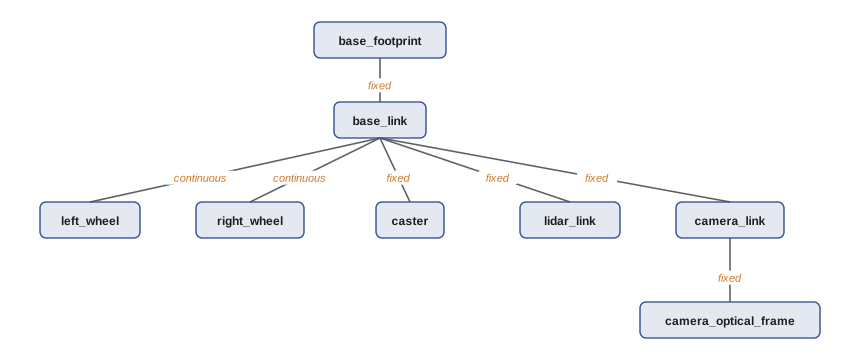
SDF and simulator-specific descriptions
URDF was designed for describing a single robot for ROS tools, and it has limits: it cannot describe closed kinematic loops, worlds with many models, lights, terrain or detailed physics properties. The Simulation Description Format (SDF), used natively by Gazebo, covers all of these. In practice teams keep the URDF (generated from Xacro) as the single source of truth for the robot, and Gazebo converts it to SDF when the robot is spawned, with simulator-specific details such as friction coefficients, sensor plugins and the ros2_control plugin added through extension tags. Worlds, buildings and obstacles are written directly in SDF. Other simulators use their own formats, such as MJCF for MuJoCo and USD for Isaac Sim, with importers for URDF.
Mass, center of mass and inertia
Wrong inertial values are one of the most common causes of unrealistic simulations: robots that tip over too easily, arms that oscillate, wheels that spin up instantly. Every link needs a positive mass and a physically consistent inertia tensor, with principal moments that satisfy the triangle inequality (each at most the sum of the other two). The best source is the CAD model, which can export mass properties from material densities. For simple shapes, standard formulas give good approximations.
# Inertia of simple shapes about their CoM (kg m^2)
def box(m, x, y, z):
    return (m * (y*y + z*z) / 12, m * (x*x + z*z) / 12, m * (x*x + y*y) / 12)
def cylinder_z(m, r, h):          # axis along z
    ixx = m * (3*r*r + h*h) / 12
    return (ixx, ixx, m * r * r / 2)
def check(I):
    a, b, c = I
    return a > 0 and b > 0 and c > 0 and a <= b + c and b <= a + c and c <= a + b
chassis = box(18.0, 0.60, 0.45, 0.20)
wheel = cylinder_z(1.2, 0.08, 0.04)
print("chassis ixx, iyy, izz = %.4f, %.4f, %.4f  valid=%s" % (*chassis, check(chassis)))
print("wheel   ixx, iyy, izz = %.5f, %.5f, %.5f  valid=%s" % (*wheel, check(wheel)))
bad = (0.01, 0.01, 0.05)          # a typo: izz too large for the others
print("typo tensor valid =", check(bad))
# parallel axis theorem: wheel spinning about the robot's vertical axis, offset 0.21 m sideways
d = 0.21
print("wheel izz about robot vertical axis = %.4f" % (wheel[0] + 1.2 * d * d))chassis ixx, iyy, izz = 0.3638, 0.6000, 0.8438 valid=True wheel ixx, iyy, izz = 0.00208, 0.00208, 0.00384 valid=True typo tensor valid = False wheel izz about robot vertical axis = 0.0550
Inertia is expressed in the link's own frame. In the Xacro listing, the joint's rotation of −π/2 about x turns the wheel link so that its z axis points sideways, along the robot's y axis; the cylinder therefore stays aligned with the link's z axis, and izz carries the larger value m r²/2 while ixx and iyy take the other moment. Mixing up the link frame and the robot frame is a classic error that gives wheels the wrong spin inertia. Tools such as the Gazebo inertia visualization, which draws an equivalent box for each link, make such mistakes easy to spot.
Worked problem
Will the robot tip when it brakes?
A simulated delivery robot has its center of mass 0.45 m above the floor and its front wheels 0.25 m ahead of the center of mass. What braking deceleration tips it forward? What if a modeling error places the center of mass at 0.30 m?
Show solution
- Tipping begins when the inertial force moment exceeds the weight moment about the front contact: \( m a h > m g d \), so \( a > g d / h \).
- With h = 0.45 m: \( a > 9.81 \times 0.25 / 0.45 \approx 5.5 \) m/s².
- With the erroneous h = 0.30 m: \( a > 9.81 \times 0.25 / 0.30 \approx 8.2 \) m/s².
Answer: The real robot tips above about 5.5 m/s², but the mismodelled one tolerates 8.2 m/s², so a simulated emergency-stop test would wrongly pass. Center-of-mass height should come from CAD or a measurement, not a guess.
Collision geometry versus visual geometry
Visual geometry is for appearance and can use detailed meshes. Collision geometry is used by the physics engine and should be as simple as possible: boxes, cylinders, spheres and capsules, or convex hulls of meshes, because collision checking cost grows with complexity and concave meshes are poorly supported by many solvers. A wheel modeled as a detailed tire mesh may bounce and jitter; modeled as a cylinder or sphere it rolls smoothly. Simplified collision shapes should still be slightly conservative where it matters for safety, such as the outline of the robot body near people.
| Element | Visual geometry | Collision geometry |
|---|---|---|
| Chassis | Detailed CAD mesh with fillets | One or two boxes |
| Wheel | Tire mesh with tread | Cylinder (or sphere for casters) |
| Lidar | Branded housing mesh | Short cylinder |
| Arm link | Smooth cast shape | Capsule or convex hull |
| Shelving in the world | Textured mesh | Boxes for uprights and shelves |
Sensor models and noise
Simulated sensors in Gazebo are added through sensor elements and plugins: cameras, depth cameras, gpu_lidar, IMU, contact, force-torque, GPS (navsat), magnetometer, altimeter and others. Each has parameters for rate, resolution, field of view and range, and most support noise models, typically additive Gaussian noise with a mean and standard deviation, sometimes with bias and bias drift. Noise-free sensors are a trap: algorithms tuned on perfect data often fail on real data, and some failure modes, such as a localization filter becoming overconfident, only appear with realistic noise.
Good sensor models go beyond Gaussian noise where it matters: lidar dropouts on dark or shiny surfaces, multipath and range spikes, rolling-shutter and motion blur in cameras, IMU bias that changes with temperature, GPS outages near buildings and wheel encoder slip. The parameters should come from datasheets and, better, from measurements of the actual sensors, the same characterization used in ROB-220 and ROB-310.
import random, math
# A simple lidar range model: Gaussian noise, dropouts on dark surfaces, occasional spikes
rnd = random.Random(42)
def lidar_range(true_r, dark=False, sigma=0.015, p_drop=0.02, p_spike=0.005, r_max=12.0):
    if dark: p_drop = 0.25                 # dark material returns fail more often
    u = rnd.random()
    if u < p_drop: return float("inf")     # no return
    if u < p_drop + p_spike: return rnd.uniform(0.1, true_r)   # spurious short return
    return min(r_max, rnd.gauss(true_r, sigma))
for dark in (False, True):
    rs = [lidar_range(4.0, dark) for _ in range(5000)]
    valid = [r for r in rs if math.isfinite(r)]
    mean = sum(valid) / len(valid)
    sd = (sum((r - mean) ** 2 for r in valid) / len(valid)) ** 0.5
print(f"dark={dark}: valid {len(valid) / len(rs):.1%}, mean {mean:.3f} m, std {sd:.3f} m")dark=False: valid 97.8%, mean 3.993 m, std 0.130 m dark=True: valid 75.0%, mean 3.984 m, std 0.203 m
The standard deviation of the valid returns is much larger than the 1.5 cm Gaussian noise because the rare spurious short returns are counted in it. This is exactly the kind of outlier behavior that robust estimators and gating (ROB-310) must handle, and a simulation that omits it gives a false sense of security.
Worked problem
Matching a noise parameter to data
A real lidar is placed 3.000 m from a flat white wall and 1000 readings are logged. Their standard deviation is 0.012 m and their mean 3.006 m. What Gaussian noise parameters should the simulated sensor use?
Show solution
- Bias: \( 3.006 - 3.000 = 0.006 \) m.
- Standard deviation: 0.012 m.
- Repeat at several ranges and surfaces; if the deviation grows with range, model it as a function of range, and add dropout rates for dark surfaces measured the same way.
Answer: Mean 0.006 m and standard deviation 0.012 m at 3 m, refined with measurements at other ranges and materials. Measured parameters are far better than datasheet typical values.
Building worlds and scenarios
A world is the environment: buildings, floors, furniture, lighting, other agents and weather. Worlds can be modeled from floor plans, built from asset libraries such as Gazebo Fuel, or generated procedurally to create many variations. A scenario is a world plus a script of what happens: start pose, goal, people walking across, a pallet appearing in an aisle, the network dropping. Scenario lists come directly from the use cases and exception flows of lesson 2, so that each requirement has simulated tests that exercise it.
Moving agents make scenarios much more valuable. Gazebo supports actors with scripted trajectories and animations; pedestrian simulation libraries add crowd behavior. Parameterized scenarios let one description generate many test cases: a person crossing at a random point, speed and angle within stated ranges. Lesson 8 extends this idea to domain randomization, where variation is used deliberately to make software robust to the gap between simulation and reality.
Worked problem
How many scenario variations?
A crossing scenario has four parameters: person speed (3 values), crossing angle (4 values), robot speed (3 values) and lighting (2 values). How many combinations are there in a full grid, and how many runs does a pairwise design need at minimum?
Show solution
- Full grid: \( 3 \times 4 \times 3 \times 2 = 72 \) runs.
- A pairwise (all-pairs) design covers every pair of parameter values at least once; its minimum size is at least the product of the two largest factor sizes, \( 4 \times 3 = 12 \).
- Pairwise tools usually find designs close to that bound, often 12 to 14 runs here.
Answer: 72 runs for the full grid against about 12 to 14 for pairwise coverage. Pairwise designs are a cheap way to catch most interaction bugs before running the full grid or random sampling.
Common mistakes
MistakeLeaving default or zero inertia on links
InsteadUse CAD mass properties or shape formulas, and check the triangle inequality.
MistakeUsing detailed visual meshes as collision geometry
InsteadUse simple primitives or convex hulls for collisions.
MistakeSimulating perfect, noise-free sensors
InsteadAdd measured noise, bias, dropouts and outliers.
MistakeKeeping separate, hand-edited URDF and SDF copies of the robot
InsteadGenerate everything from one Xacro source and add simulator extensions.
MistakeTesting only in an empty world
InsteadBuild scenarios from use cases and exception flows, with moving agents and variations.
Summary and key terms
- URDF describes a robot as a tree of links and joints with visual, collision and inertial properties; Xacro adds macros and properties.
- SDF describes complete worlds and simulator details; teams keep one Xacro source and add simulator extensions.
- Mass, center of mass and inertia must be realistic and consistent, ideally from CAD, or dynamics such as tipping will be wrong.
- Collision geometry should be simple and conservative where safety matters; visual geometry can be detailed.
- Sensor models need measured noise, bias, dropouts and outliers, not perfect data.
- Worlds and scenarios should come from use cases and exception flows and include moving agents.
- Parameterized scenarios and designs such as pairwise testing generate many useful cases cheaply.
- URDF
- The Unified Robot Description Format, an XML description of links and joints.
- Xacro
- An XML macro language that generates URDF from reusable, parameterized pieces.
- SDF
- The Simulation Description Format used by Gazebo for robots and worlds.
- Link
- A rigid body in a robot description.
- Joint
- A connection between two links with a type, axis and limits.
- Inertia tensor
- A 3 × 3 matrix describing a body's resistance to rotational acceleration.
- Collision geometry
- Simplified shapes used by the physics engine for contact.
- Sensor plugin
- Simulator code that generates sensor data and publishes it.
- Actor
- A scripted moving agent, such as a walking person, in a simulated world.
- Pairwise testing
- A test design that covers every pair of parameter values at least once.
Practice problems
Work each problem on paper first, then reveal the answer to check.
What three kinds of property can a URDF link have?
Show answer
Visual, collision and inertial.
Name four URDF joint types.
Show answer
For example fixed, revolute, continuous and prismatic.
Why use Xacro?
Show answer
To avoid repetition with macros, properties and expressions.
What can SDF describe that URDF cannot?
Show answer
Worlds, lights, closed loops and detailed physics settings.
What is the inertia of a solid cylinder about its axis?
Show answer
\( m r^2 / 2 \).
What inequality must principal moments satisfy?
Show answer
Each must be at most the sum of the other two.
Why simplify collision geometry?
Show answer
Collision checking is faster and more stable with simple convex shapes.
Name two sensor effects beyond Gaussian noise.
Show answer
For example dropouts and spurious short returns.
Where should scenario lists come from?
Show answer
From use cases and exception flows in the requirements.
How many runs does a full grid of 2 × 3 × 5 values need?
Show answer
30.
Lesson quiz · 5 questions
Score 60% or more to complete this lesson.
Create a free account to save your progress, take quizzes and earn a certificate.