
PMP-131 · Lesson 4 of 12 · 27 min
Qualitative and quantitative risk analysis
Identification produces a list; analysis turns it into priorities and numbers. Qualitative analysis ranks individual risks quickly using probability, impact and other characteristics, so that attention goes to the risks that matter. Quantitative analysis models the combined effect of risks and estimate uncertainty on project objectives, producing results such as the probability of finishing within budget. This lesson applies both to Project Compass, including expected monetary value, a decision tree, a Monte Carlo cost simulation and a sensitivity (tornado) analysis. PMP-130 already showed a Monte Carlo schedule analysis; here the focus is on cost and on how the results feed decisions about reserves.
Qualitative analysis: probability and impact
Qualitative analysis assesses each risk's probability of occurring and its impact on objectives if it does, using the scales defined in the risk management plan. Defining the scales matters, because without definitions one person's "high" is another's "medium". Scales are usually ordinal (very low to very high) with numeric ranges attached, and impact is defined separately for each objective.
| Score | Probability | Cost impact | Schedule impact (opening date) | Quality impact |
|---|---|---|---|---|
| 1 Very low | Below 10 % | Under $10,000 | Under 2 working days | Barely noticeable |
| 2 Low | 10 % to 30 % | $10,000 to $40,000 | 2 to 5 days | Minor; only demanding users notice |
| 3 Medium | 30 % to 50 % | $40,000 to $80,000 | 5 to 10 days | Visible to patrons; needs sponsor approval |
| 4 High | 50 % to 70 % | $80,000 to $150,000 | 10 to 20 days | Unacceptable to the sponsor |
| 5 Very high | Above 70 % | Over $150,000 | Over 20 days | Deliverable effectively unusable |
A probability and impact matrix combines the two scores into a priority. Project Compass uses score = probability × impact, with 12 or more treated as high, 6 to 10 as medium and 5 or less as low. Some organizations weight impact more heavily than probability, so that unlikely but catastrophic risks are not dismissed; others use an asymmetric matrix. The exam does not require a particular scheme, only that the scheme is defined in advance and applied consistently.
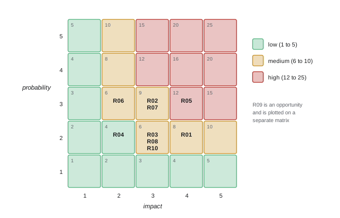
Probability and impact are not the only useful characteristics. Urgency (or proximity) is how soon a response must be in place to be effective: the permit risk must be addressed now, while the app store rework risk is months away. Detectability is how easy it is to see the risk coming. Connectivity is how many other risks a risk is linked to; strategic impact is its effect on the organization's goals. Many teams also rate the quality of the risk data: a risk scored on guesswork with little understanding should be investigated further before it is relied on. A bubble chart can show three dimensions at once, for example probability, impact and urgency as bubble size.
Qualitative analysis has well-known weaknesses. Ordinal scores cannot properly be multiplied or added, so a score of 12 is not "twice as risky" as 6. Scorers anchor on one another and on early impressions. And a register of individually medium risks can still hide a large overall risk. These are reasons to use qualitative scores for ranking and conversation, and quantitative methods when decisions about money and dates depend on the answer.
Expected monetary value
Expected monetary value (EMV) is the probability of a risk multiplied by its monetary impact, with threats negative and opportunities positive. Summed over a set of risks, it gives the average outcome you would expect if the situation could be repeated many times. PMP-130 used it to size the Project Compass contingency reserve.
# Expected monetary value of the four costed risks and the opportunity ($000)
items = [("R01 asbestos in ceiling", 0.25, -120), ("R02 permit delay costs", 0.40, -60),
         ("R03 tag price increase", 0.30, -50), ("R04 app store rework", 0.25, -44),
         ("R09 joint tag order discount", 0.50, +18)]
threats = 0
for name, p, impact in items:
    emv = p * impact
    print(f"{name:30s} p={p:.2f}  impact {impact:+5d}  EMV {emv:+7.1f}")
    if impact < 0:
        threats += emv
opp = sum(p * i for _, p, i in items if i > 0)
print(f"\nThreat EMV {threats:+.0f}  ->  contingency reserve {-threats:.0f}")
print(f"Opportunity EMV {opp:+.0f} (not netted off; pursued as a response, see lesson 5)")R01 asbestos in ceiling p=0.25 impact -120 EMV -30.0 R02 permit delay costs p=0.40 impact -60 EMV -24.0 R03 tag price increase p=0.30 impact -50 EMV -15.0 R04 app store rework p=0.25 impact -44 EMV -11.0 R09 joint tag order discount p=0.50 impact +18 EMV +9.0 Threat EMV -80 -> contingency reserve 80 Opportunity EMV +9 (not netted off; pursued as a response, see lesson 5)
The four costed threats have a combined EMV of −$80,000, which is the contingency reserve in the cost baseline. The joint tag order opportunity has an EMV of +$9,000. The library chose not to reduce the contingency by the opportunity's value, because the opportunity was still uncertain and the board preferred to treat any saving as a bonus; lesson 5 shows how the team pursued it actively instead. Note what EMV is not: no single outcome will equal $80,000. If asbestos is found, the cost is $120,000 for that risk alone. EMV is an average for planning reserves across many risks, not a prediction of what will happen.
Decision trees
A decision tree models a decision with uncertain outcomes. Squares are decision nodes, circles are chance nodes and the branches carry probabilities and values. The EMV of each chance node is calculated from right to left by multiplying outcomes by probabilities, and at each decision node the branch with the best EMV is chosen, a process called rolling back the tree. Costs incurred on a branch, such as the cost of a survey, are subtracted along that branch.
# Decision tree: add an intrusive survey of the concealed ceiling space before demolition? ($000)
# (The basic pre-demolition hazardous materials assessment is required anyway; this is an extra.)
survey_cost = 8
# Without survey: 25 % chance asbestos is found mid-demolition (abatement 80 + delay 40)
no_survey = 0.25 * -(80 + 40) + 0.75 * 0
# With survey: if found early (25 %), abatement is planned before work starts: 80, no delay
with_survey = -survey_cost + 0.25 * -80 + 0.75 * 0
print(f"EMV without survey: {no_survey:.0f}")
print(f"EMV with survey:    {with_survey:.0f}")
print("Choose:", "survey" if with_survey > no_survey else "no survey",
      f"(advantage {abs(with_survey - no_survey):.0f})")
# Sensitivity: at what probability of asbestos does the survey stop paying for itself?
for p in (0.05, 0.10, 0.15, 0.20, 0.25, 0.30):
    a = p * -120; b = -survey_cost + p * -80
print(f" p={p:.2f}: no survey {a:6.1f} survey {b:6.1f} -> {'survey' if b > a else 'no survey'}")EMV without survey: -30 EMV with survey: -28 Choose: survey (advantage 2) p=0.05: no survey -6.0 survey -12.0 -> no survey p=0.10: no survey -12.0 survey -16.0 -> no survey p=0.15: no survey -18.0 survey -20.0 -> no survey p=0.20: no survey -24.0 survey -24.0 -> no survey p=0.25: no survey -30.0 survey -28.0 -> survey p=0.30: no survey -36.0 survey -32.0 -> survey
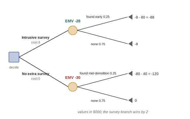
A basic hazardous materials assessment is required before demolition anyway, and it found no asbestos in accessible areas. The open question was whether to pay $8,000 for an intrusive survey of the concealed space above the old ceiling. Without it, there is a 25 % chance of finding asbestos mid-demolition, costing $80,000 for abatement plus $40,000 of delay. With it, asbestos would be found before work starts, so the abatement could be planned without delay. The survey branch has an EMV of −$28,000 against −$30,000 without, a narrow advantage of $2,000. The sensitivity table shows why the decision is close: below a 20 % probability, the survey does not pay for itself in money alone.
The team commissioned the survey, and the reason illustrates the limits of EMV. Money is not the only consideration: discovering asbestos mid-demolition would expose workers and halt the critical path, and the library's appetite for safety and opening-date risk is low. A decision maker who is risk-averse may reasonably pay slightly more than the EMV-optimal amount to avoid a bad outcome. Exam questions usually ask for the EMV-based answer, but real decisions weigh EMV alongside risk appetite, safety and reputation.
Quantitative analysis: Monte Carlo simulation
Qualitative scores and EMV look at risks one at a time. Monte Carlo simulation looks at the whole: it represents uncertain estimates as probability distributions, adds discrete risk events with their probabilities, and recalculates the total thousands of times, each time drawing random values. The result is a distribution of possible outcomes, from which you can read the probability of meeting a target and the value associated with any confidence level. PMP-130 applied this to the fit-out schedule (P50 about 108 working days, P80 about 114). Here it is applied to cost.
# Monte Carlo cost risk for Project Compass ($000): estimate uncertainty plus risk events
import random
random.seed(131)
# Major cost groups: (low, most likely, high) from the estimators; sum of most likely = 2,320
groups = {"Design and permits": (140, 150, 175), "Construction": (1080, 1150, 1320),
          "Furniture and fixtures": (300, 320, 360), "RFID and kiosks": (330, 350, 410),
          "Mobile app": (190, 210, 260), "Transition": (130, 140, 160)}
risks = [(0.25, 120), (0.40, 60), (0.30, 50), (0.25, 44)]
N = 20000
totals = []
for _ in range(N):
    t = sum(random.triangular(lo, hi, ml) for lo, ml, hi in groups.values())
    t += sum(imp for p, imp in risks if random.random() < p)
    totals.append(t)
totals.sort()
pct = lambda q: totals[int(q * N) - 1]
print(f"Point estimate (most likely, no risks): {sum(v[1] for v in groups.values()):,}")
print(f"Mean {sum(totals) / N:,.0f}   P50 {pct(0.50):,.0f}   P80 {pct(0.80):,.0f}   P90 {pct(0.90):,.0f}")
for target in (2320, 2400, 2520):
    share = sum(t <= target for t in totals) / N
print(f"P(cost <= {target:,}) = {share:.0%}")Point estimate (most likely, no risks): 2,320 Mean 2,472 P50 2,465 P80 2,547 P90 2,589 P(cost <= 2,320) = 2% P(cost <= 2,400) = 22% P(cost <= 2,520) = 72%
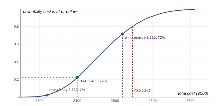
The results are sobering. The sum of the most likely estimates, $2.32 million, is achieved in only about 2 % of trials, because the estimates are right-skewed: the high values are further from the most likely than the low values are, so the averages sit above the most likely figures. The cost baseline of $2.4 million, which adds the $80,000 EMV contingency, has only about a 22 % chance of being enough. The full budget including the $120,000 management reserve, $2.52 million, gives about 72 % confidence, and P80 is about $2.55 million.
This is the overall project risk that the risk register alone did not show. EMV contingency covered the four listed risk events on average, but not the uncertainty in every estimate. The project manager presented these results at the baseline review. The board had a firm funding cap and kept the baseline at $2.4 million with the 5 % management reserve, but it recorded that the budget's confidence level was low and asked for early warning if the forecast trended upwards. PMP-130's month 6 earned value analysis, with a forecast of about $2.6 million, is exactly the warning the simulation predicted. Decisions made with honest confidence levels lead to better conversations later than decisions made on single-point estimates.
Quantitative analysis needs care. Results are only as good as the input distributions, and correlations matter: if construction costs run high because of a hot labour market, furniture installation probably runs high too, and ignoring that correlation understates the spread. Simulation is worth the effort on large, complex or high-stakes projects, or where a contract or funding decision depends on confidence levels; on small projects, qualitative analysis may be enough.
Sensitivity analysis and tornado diagrams
Sensitivity analysis asks which uncertainties drive the result. A tornado diagram shows, for each uncertain input, how much the outcome swings when that input moves from its low to its high value with everything else held at the base case. The longest bar goes at the top, giving the funnel shape that gives the chart its name.
# Tornado (one-at-a-time sensitivity): swing in total cost when each group goes low to high ($000)
groups = {"Design and permits": (140, 150, 175), "Construction": (1080, 1150, 1320),
          "Furniture and fixtures": (300, 320, 360), "RFID and kiosks": (330, 350, 410),
          "Mobile app": (190, 210, 260), "Transition": (130, 140, 160)}
base = sum(ml for _, ml, _ in groups.values())
rows = []
for name, (lo, ml, hi) in groups.items():
    rows.append((hi - lo, name, base - ml + lo, base - ml + hi))
print(f"Base case {base:,}")
for swing, name, low, high in sorted(rows, reverse=True):
    bar = "#" * round(swing / 10)
print(f"{name:24s}{low:6,} to {high:6,} swing {swing:4d} {bar}")Base case 2,320 Construction 2,250 to 2,490 swing 240 ######################## RFID and kiosks 2,300 to 2,380 swing 80 ######## Mobile app 2,300 to 2,370 swing 70 ####### Furniture and fixtures 2,300 to 2,360 swing 60 ###### Design and permits 2,310 to 2,345 swing 35 #### Transition 2,310 to 2,340 swing 30 ###
Construction dominates, with a swing of $240,000, three times the next largest. That tells the project manager where to spend risk management effort: firming up construction costs through a more detailed estimate, earlier contractor involvement or a contract type that shares risk (lesson 8) will reduce overall uncertainty far more than refining the transition budget. Monte Carlo tools often produce a similar ranking from the correlation between each input and the total, which also accounts for the shape of each distribution.
Worked problem
Expected monetary value with an opportunity
A different project has three risks: a 30 % chance of a supplier delay costing $50,000, a 10 % chance of a regulatory change costing $120,000 and a 40 % chance of a bulk purchase discount saving $20,000. What is the total EMV, and how much contingency would cover the threats?
Show solution
- Supplier delay: 0.30 × −50,000 = −$15,000.
- Regulatory change: 0.10 × −120,000 = −$12,000.
- Discount: 0.40 × +20,000 = +$8,000.
- Total EMV = −15,000 − 12,000 + 8,000 = −$19,000. Threat EMV alone is −$27,000.
Answer: Total EMV is −$19,000. A contingency of $27,000 covers the threats on average; netting off the opportunity would give $19,000, which assumes the opportunity is pursued and is reasonably likely.
Common mistakes
MistakeScoring risks without defined probability and impact scales.
InsteadUse the scales and matrix defined in the risk management plan.
MistakeTreating EMV as the amount a risk will cost.
InsteadEMV is a probability-weighted average used for comparing options and sizing reserves.
MistakeAssuming the sum of most likely estimates is the likely total cost.
InsteadSkewed estimates and risks push the likely total higher; simulation shows the confidence level.
MistakeForgetting to subtract the cost of a decision branch in a decision tree.
InsteadInclude branch costs and roll back from right to left.
MistakeSpreading risk effort evenly across all cost items.
InsteadUse sensitivity analysis to focus on the inputs that drive the outcome.
Summary and key terms
- Qualitative analysis ranks risks by probability and impact using defined scales and a matrix, plus urgency and other factors.
- Ordinal scores are for ranking; quantitative methods support decisions about money and dates.
- EMV = probability × impact; threats negative, opportunities positive; summed EMV sizes contingency.
- Decision trees roll back from right to left, choosing the branch with the best EMV after branch costs.
- Monte Carlo simulation shows overall project risk: the probability of meeting a target and values at P50 or P80.
- Tornado diagrams rank the uncertainties that drive the result.
- Risk appetite, safety and reputation can justify decisions that differ from pure EMV.
- Qualitative risk analysis
- Prioritizing individual risks by assessing probability, impact and other characteristics.
- Quantitative risk analysis
- Numerically analysing the combined effect of risks and uncertainty on objectives.
- Probability and impact matrix
- A grid mapping probability against impact to assign priority.
- Expected monetary value
- The probability-weighted average of the monetary outcomes of a risk or decision.
- Decision tree
- A diagram that evaluates alternatives with uncertain outcomes by EMV.
- Monte Carlo simulation
- Repeated random sampling from input distributions to produce a distribution of outcomes.
- Tornado diagram
- A sensitivity chart showing the swing in an outcome caused by each input, largest at the top.
- Urgency
- How soon a response to a risk must be implemented to be effective.
Practice problems
Work each problem on paper first, then reveal the answer to check.
A risk has a 20 % probability and a $90,000 cost impact. What is its EMV?
Show answer
−$18,000.
An opportunity has a 60 % chance of saving $10,000. EMV?
Show answer
+$6,000.
Which direction do you calculate a decision tree?
Show answer
From right to left (rolling back).
What does P80 mean in a cost simulation?
Show answer
There is an 80 % probability the cost will be at or below that value.
Which chart shows which input uncertainty matters most?
Show answer
A tornado diagram.
Why do skewed estimates make the most likely total unlikely?
Show answer
High outcomes are further from the mode than low ones, so averages and totals shift upwards.
What is urgency in qualitative analysis?
Show answer
How soon a response must be in place to be effective.
Where does the board find the confidence level of the budget?
Show answer
From quantitative analysis such as a Monte Carlo simulation.
Can ordinal risk scores be meaningfully added across risks?
Show answer
Not really; they are for ranking, not arithmetic.
A decision tree branch costs $8,000 to take. How is that handled?
Show answer
Subtract it along that branch before comparing EMVs.
Lesson quiz · 5 questions
Score 60% or more to complete this lesson.
Create a free account to save your progress, take quizzes and earn a certificate.