
ROB-100 · Lesson 7 of 12 · 25 min
Control: from feedback loops to autonomy
Control is how a robot makes its actuators do what its software wants. A command such as drive at 1 m/s, hold this joint at 45° or hover at 10 m sounds simple, but motors respond with delays, loads change, wheels slip, wind gusts and batteries sag. Control engineering provides the methods that let a robot reach and hold its targets despite these disturbances, and the same feedback idea scales up from a single motor to a robot that decides on its own where to go. This lesson starts with the difference between open-loop and closed-loop control, works through a proportional controller step by step, introduces the widely used PID controller and the ideas of stability and tuning, explains how robots stack control loops in layers, and ends with how higher levels of decision-making give robots autonomy, including the levels used to describe automated driving.
Open-loop and closed-loop control
In open-loop control, the controller sends a command without checking the result. A toaster heats for a set time whatever the colour of the bread; a stepper motor is commanded a number of steps and assumed to have moved that far. Open-loop control is simple and works well when the system is predictable and disturbances are small, but it cannot correct errors it does not know about. In closed-loop, or feedback, control, a sensor measures the actual output, the controller compares it with the desired value, called the setpoint or reference, and adjusts its command to reduce the difference, called the error. A thermostat is the classic example: it turns the heat on when the room is colder than the setpoint and off when it is warmer. In robots, closed-loop control holds wheel speeds, joint angles, arm forces, drone attitude and the robot's path.
Here \( r(t) \) is the setpoint, \( y(t) \) the measured output and \( e(t) \) the error at time \( t \). Every feedback controller is some rule for turning the error into a command.
The proportional controller
The simplest useful feedback rule is proportional control: make the command proportional to the error. If the error is large, push hard; as the error shrinks, push gently. Written as an equation, the command is \( u = K_p e \), where \( K_p \) is the proportional gain, a number the engineer chooses. A larger gain responds more strongly. Proportional control is easy to understand by working through it step by step, as a robot's computer does in each cycle of its control loop.
Worked problem
A proportional controller, one step at a time
A robot is 2.0 m from a wall and must stop 0.5 m from it. Its controller runs every 0.1 s and commands a speed proportional to the remaining distance error, with gain 1.0 s⁻¹, so speed = 1.0 × error. Assume the robot instantly reaches each commanded speed. Trace the first four control steps.
Show solution
- Step 1: error \( = 2.0 - 0.5 = 1.5 \) m; speed 1.5 m/s; it moves \( 1.5 \times 0.1 = 0.15 \) m, leaving 1.85 m to the wall.
- Step 2: error \( = 1.35 \) m; speed 1.35 m/s; moves 0.135 m, leaving 1.715 m.
- Step 3: error \( = 1.215 \) m; moves 0.1215 m, leaving about 1.594 m.
- Step 4: error \( \approx 1.094 \) m; moves about 0.109 m, leaving about 1.484 m.
- Each step removes 10 % of the remaining error, so the robot slows smoothly as it approaches and never crosses the 0.5 m line in this ideal model.
Answer: About 1.48 m from the wall after four steps, with the error shrinking by 10 % per step.
In this ideal example, each step multiplies the error by \( 1 - K_p \Delta t = 0.9 \), so the error decays geometrically. If the gain were 10 s⁻¹, the factor would be \( 1 - 10 \times 0.1 = 0 \), and the robot would reach the target in one step; at 15 s⁻¹ the factor would be −0.5 and it would overshoot and come back; above 20 s⁻¹ the factor's size would exceed 1 and the robot would oscillate with growing swings. Real robots have inertia and delays, so they become unstable at much lower gains than this idealized model suggests, but the lesson holds: too little gain is sluggish, too much causes overshoot, oscillation and eventually instability.
PID control
Proportional control has a common weakness: when there is a steady disturbance, such as a robot climbing a slope or an arm holding a heavy load, a small error is needed to produce the command that balances it, so the system settles slightly off target. This leftover error is called steady-state error. The PID controller, short for proportional-integral-derivative, adds two more terms. The integral term adds up the error over time, so even a small persistent error eventually builds a large correction, removing steady-state error. The derivative term responds to how fast the error is changing, acting like a damper that slows the approach and reduces overshoot. PID controllers are by far the most widely used controllers in industry and robotics: they run in motor drives, joint controllers, drone flight controllers and countless machines.
Each term has its own gain, \( K_p \), \( K_i \) and \( K_d \). In software the integral is a running sum of error times the time step, and the derivative is the change in error divided by the time step. Practical PID code also limits the integral so it does not grow huge when an actuator is saturated, a problem called integrator wind-up, and often filters the derivative, because differentiating noisy sensor data amplifies the noise.
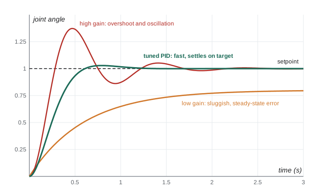
Describing performance and tuning
Engineers describe how well a controller responds to a sudden change in setpoint, called a step, with a few standard measures. Rise time is how long the output takes to go from 10 % to 90 % of the way to the new setpoint. Overshoot is how far it goes past the setpoint, as a percentage of the step. Settling time is how long it takes to stay within a small band, often 2 %, of the setpoint. Steady-state error is the difference that remains after it settles. There are trade-offs: faster response generally brings more overshoot, and a system tuned for one load may behave poorly with another.
Tuning means choosing the gains. In practice, engineers often start with only proportional gain, increase it until the response is quick but begins to overshoot or oscillate, then add derivative gain to damp the overshoot and integral gain to remove steady-state error, testing carefully at each step. Systematic methods, such as the Ziegler–Nichols rules and model-based design using a mathematical model of the robot, give better starting points, and many motor drives have automatic tuning functions. Testing at low speed, with limits and emergency stops ready, is essential, because an unstable controller can make a robot swing violently.
| Effect of increasing | Rise time | Overshoot | Steady-state error | Risk |
|---|---|---|---|---|
| Proportional gain Kp | Faster | Increases | Decreases but remains | Oscillation |
| Integral gain Ki | Faster | Increases | Eliminated | Wind-up, slow oscillation |
| Derivative gain Kd | Little change | Decreases | Little change | Amplifies noise |
Control in layers
Robots almost always use several control loops nested inside one another, each running at its own rate. In a robot arm, the innermost loop in each motor drive controls the motor current, and therefore torque, thousands of times a second; around it, a velocity loop and a position loop hold each joint on its commanded trajectory; above those, a trajectory generator works out smooth paths for all the joints at once; and above that, the robot program or a motion planner decides where the tool should go. A drone's flight controller runs an attitude loop, holding roll, pitch and yaw, hundreds of times a second, inside a slower position and velocity loop that follows a planned path. Inner loops must be faster than outer ones, so that from the outer loop's point of view, the inner loop has already done its job. This layered structure lets each loop be designed and tested separately.
Beyond PID
Many more advanced control methods are used in robotics and covered later in the program. Feedforward control uses a model to predict the command needed, such as the torque to accelerate a known mass, and adds it to the feedback, so the feedback loop only corrects small errors. State-feedback methods such as the linear-quadratic regulator use all the measured variables of a system at once. Model predictive control repeatedly optimizes a short plan of future commands, taking limits into account, and is widely used in autonomous vehicles and legged robots. Impedance and force control let a robot behave like a spring, yielding when it touches something, which is essential for contact tasks and for safety near people. Increasingly, learned controllers trained with reinforcement learning in simulation drive legged robots and robot hands.
From control to autonomy
Feedback control keeps a robot on a commanded path; autonomy is about deciding what that path should be. Above the control layers, an autonomous robot needs to estimate its state and its surroundings, decide on goals or accept them from people, plan how to achieve them, monitor progress and handle problems, such as replanning around a blocked aisle or asking for help when stuck. Each of these is itself a kind of feedback loop, comparing what the robot intended with what is happening, but working with richer information over longer time scales. The next lesson describes how robot software is organized to do this.
For automated driving, a widely used scale from SAE International's J3016 standard describes six levels of driving automation. Levels 0 to 2 cover driver support, such as warnings, adaptive cruise control and lane centring, where the human must supervise at all times. At Level 3, the system drives in certain conditions and the human must take over when asked. At Level 4, the system drives itself within a defined operational design domain, such as particular city areas and weather conditions, with no expectation that a person will take over. Level 5 would drive anywhere a human could, and does not exist today. Driverless taxi services, which by 2026 were providing hundreds of thousands of paid rides each week in several US cities, operate at Level 4 within their service areas. The idea of an operational design domain, the conditions in which an autonomous system is designed to work safely, applies to robots of every kind.
Feedback control is everywhere in everyday robots. A robot vacuum holds its wheel speeds with encoder feedback, follows walls by keeping a side sensor reading constant, and steers back to its dock by centring an infrared beacon. A drone holds itself level with a fast attitude loop and its altitude with a barometer and range sensor. A collaborative arm detects a collision when the measured joint torque differs from what its dynamic model predicts, and stops. Recognizing the setpoint, the measurement, the error and the controller in each case is a good way to understand any robot.
Control engineers also think carefully about what happens when things go wrong. A controller should behave sensibly if a sensor fails, a wheel slips or a motor reaches its limit: commands are clamped to safe ranges, sudden jumps in the setpoint are smoothed, and watchdog timers stop the motors if the control loop stops running. Designing for these cases is as important as tuning for normal operation.
Common mistakes
MistakeUsing open-loop control where disturbances matter.
InsteadClose the loop with sensor feedback when loads and conditions vary.
MistakeTurning up the gain to fix every problem.
InsteadRemember that high gain causes overshoot, oscillation and instability.
MistakeLetting the integral term grow while an actuator is saturated.
InsteadLimit the integral to prevent wind-up.
MistakeMaking an outer loop as fast as the inner loop.
InsteadRun inner loops much faster than the loops around them.
MistakeCalling any driver-assistance feature self-driving.
InsteadUse the SAE levels and state the operational design domain.
Summary and key terms
- Open-loop control acts without measuring the result; closed-loop control corrects the error.
- The error is the setpoint minus the measured output.
- Proportional control commands in proportion to the error; too much gain causes instability.
- PID adds integral action to remove steady-state error and derivative action to reduce overshoot.
- Rise time, overshoot, settling time and steady-state error describe performance.
- Robots nest fast inner loops inside slower outer loops.
- Autonomy adds estimation, decision-making and planning; SAE J3016 defines driving automation levels.
- Open-loop control
- Control without feedback from the output.
- Closed-loop control
- Control that uses measured output to correct errors.
- Setpoint
- The desired value of a controlled quantity.
- Error
- The setpoint minus the measured output.
- Proportional gain
- The factor relating command to error.
- PID controller
- A controller with proportional, integral and derivative terms.
- Steady-state error
- The error remaining after the response settles.
- Overshoot
- How far a response goes past its setpoint.
- Integrator wind-up
- Excessive build-up of the integral term while an actuator is saturated.
- Operational design domain
- The conditions in which an autonomous system is designed to operate.
Practice problems
Work each problem on paper first, then reveal the answer to check.
Give an example of open-loop control.
Show answer
A toaster timer or a stepper motor without an encoder.
Setpoint 90°, measured 84°. Error?
Show answer
6°.
Kp = 2 and error = 0.3 m. Command?
Show answer
0.6 (for example, m/s).
In the ideal model, Kp = 5 s⁻¹ and Δt = 0.1 s. Error factor per step?
Show answer
0.5.
What does the integral term fix?
Show answer
Steady-state error.
What does the derivative term do?
Show answer
Damps the response and reduces overshoot.
Define settling time.
Show answer
Time for the output to stay within a small band of the setpoint.
Why must inner loops be faster?
Show answer
So they have settled before the outer loop acts again.
What SAE level are today's driverless taxi services?
Show answer
Level 4, within a defined domain.
What is model predictive control?
Show answer
Repeatedly optimizing a short plan of future commands within limits.
Lesson quiz · 5 questions
Score 60% or more to complete this lesson.
Create a free account to save your progress, take quizzes and earn a certificate.