
ROB-330 · Lesson 12 of 12 · 34 min
Capstone: a perception pipeline for a pick-and-place robot
This capstone brings the course together in one design. A collaborative robot arm must pick mixed parts from a moving conveyor and place them into fixtures. Parts arrive in random positions and orientations, sometimes touching, under factory lighting that changes through the day. The robot needs, for every part, its type, its 6-D pose in the robot base frame, and a time stamp, delivered early enough to plan and execute a grasp before the part leaves reach. You will work through the design as a perception engineer would: write requirements, choose and place the camera, plan calibration, build the detection and pose pipeline, budget latency and error, plan the evaluation, and address safety and privacy. The numbers are illustrative but realistic; the method is what transfers to any robot vision task.
Requirements
Good perception design starts from what the robot must achieve, not from algorithms. The team agrees the following requirements, each testable.
| ID | Requirement | Value |
|---|---|---|
| P1 | Part types recognized | 6 types, 40 to 150 mm long |
| P2 | Pick position accuracy in the robot frame (95 % of picks) | ±2.0 mm in x and y, ±3.0 mm in z |
| P3 | Orientation accuracy about the vertical axis | ±3° |
| P4 | Conveyor speed | up to 0.25 m/s |
| P5 | Throughput | 20 picks per minute |
| P6 | Time from image capture to pose available to the planner | ≤ 120 ms |
| P7 | Pick success rate in acceptance testing | ≥ 99.0 % |
| P8 | Behaviour on low confidence | skip the part and flag it; never pick on a guess |
Two requirements deserve comment. P2 is about the whole chain, not just the camera: calibration, detection, pose estimation, time synchronization and the robot's own accuracy all contribute, so it must be split into an error budget. P8 encodes a design principle from every lesson: perception outputs must carry confidence, and the system must have a safe default when confidence is low.
Camera choice and placement
Parts lie flat on the belt, so a camera looking straight down on a section of conveyor upstream of the robot is natural: the belt is a known plane (lesson 5), which constrains the geometry, and parts are seen without occlusion by the arm. The field of view must cover the belt width of 400 mm plus margin, and the image must resolve P2.
Worked problem
Resolution needed for the accuracy requirement
The camera must see 480 mm across the belt (including margin). Experience shows the pose pipeline locates part features to about 0.5 px (1σ) after refinement. If the camera's share of the ±2.0 mm (95 %, about 2σ) budget is 0.6 mm at 1σ, what pixel footprint is needed, and how many pixels across?
Show solution
- Pixel footprint: \( 0.6 \text{ mm}/0.5 \text{ px} = 1.2 \) mm per pixel at most.
- Pixels across 480 mm: \( 480/1.2 = 400 \) px minimum.
- Add margin for detection of the smallest part (40 mm should span at least 50 px, so 0.8 mm/px): \( 480/0.8 = 600 \) px.
Answer: At least about 600 pixels across the belt. A 2448 × 2048 global-shutter camera gives roughly 0.2 mm/px over 480 mm, ample headroom, and allows binning or a region of interest if processing time is tight.
Worked problem
Choosing the lens
The camera is mounted 0.90 m above the belt with a 2448-pixel-wide sensor of 3.45 µm pixels. What focal length covers 480 mm across?
Show solution
- Sensor width: \( 2448 \times 0.00345 = 8.45 \) mm.
- From similar triangles: \( f = 8.45 \times 900/480 = 15.8 \) mm.
Answer: About 16 mm; a standard 16 mm machine-vision lens covers about 475 mm, so the camera can be raised slightly or a 12 mm lens used for more margin, with its larger distortion handled by calibration.
A global-shutter sensor is required: at 0.25 m/s a rolling shutter that reads out over 20 ms would skew parts by 5 mm (ROB-220). The exposure must also freeze motion. At 0.25 m/s and 0.2 mm per pixel, the belt moves 1.25 px per millisecond, so an exposure of 0.4 ms keeps blur to 0.5 px, which needs bright, even lighting: a diffuse LED ring or dome light strobed in sync with exposure, which also makes images consistent through the day and suppresses glare from shiny parts. Fixing exposure and gain, rather than leaving auto-exposure on, keeps detection behaviour stable. A depth camera is not needed for flat parts on a known plane, but height must be known per part type for the z coordinate, and a check for stacked or upturned parts is wise: a simple laser line or a low-cost depth sensor can flag parts whose height does not match their type.
Calibration plan
Three calibrations link pixels to robot coordinates (lesson 3).
- Intrinsics and distortion: a ChArUco board, 25 to 40 images covering the whole field with strong tilts, focus and aperture locked; accept only if RMS reprojection error is below 0.3 px and parameter uncertainties are small.
- Camera to belt plane: the homography or plane pose from a flat target lying on the belt.
- Camera to robot base: the robot touches the corners of a target on the belt with a calibrated pointer tool, or picks up a target and presents it to the camera in several poses. Verification: the robot touches ten independently measured points, and the residual must be within the budget.
- Belt motion: an encoder on the conveyor gives belt position, so each image is tagged with the encoder count at exposure and the part's position can be predicted at any later time. The encoder's scale (millimetres per count) is itself calibrated by tracking a marker over a measured distance.
A fixed fiducial at the edge of the field of view is checked every few minutes in production; if its measured position drifts by more than 0.3 mm, the cell raises an alarm for recalibration.
Detection and pose pipeline
The pipeline follows the structure of lesson 1, with each stage chosen for this task.
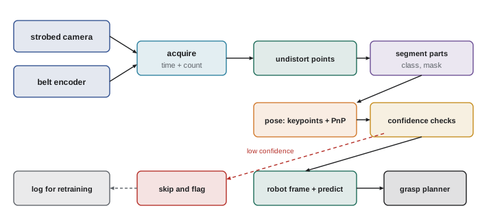
1. Acquire: strobed global-shutter image with time stamp and encoder count, triggered every 120 mm of belt travel so each part is seen at least twice.
2. Detect and segment: a small instance segmentation network (lesson 10) gives class, mask and confidence per part; touching parts are separated by their masks. It is trained on images from this cell, with labels bootstrapped by a foundation segmentation model and checked by people, augmented for lighting changes and blur, and split by production day for validation.
3. Estimate pose: for each mask, a keypoint head predicts four to eight known points on the part; their pixel coordinates are undistorted and, since the part lies on the known belt plane at a known height, PnP (lesson 11) gives position and orientation, refined by minimizing reprojection error. For symmetric parts, the orientation is reduced to the symmetry-distinct range.
4. Check: reject a part if detection confidence is below threshold, if reprojection error exceeds 1.5 px, if its measured outline does not match the model, or if consecutive observations disagree by more than 1 mm; these feed requirement P8.
5. Transform and predict: map the pose into the robot base frame with the calibrated extrinsics, and add the belt displacement since exposure using the encoder.
6. Track: associate observations of the same part across frames (lesson 11) using the predicted belt motion, averaging poses to reduce noise.
7. Log: store images of low-confidence parts and failed picks for review and retraining, addressing distribution shift (lesson 9).
Latency and motion compensation
Worked problem
Latency budget
Measured stage times (99th percentile) are: exposure and readout 9 ms, transfer 6 ms, pre-processing 4 ms, segmentation network 38 ms, keypoints and PnP for up to 6 parts 18 ms, checks and transform 3 ms, publication to the planner 2 ms. Does the pipeline meet P6, and how far does the belt move meanwhile?
Show solution
- Total: \( 9 + 6 + 4 + 38 + 18 + 3 + 2 = 80 \) ms.
- Margin against 120 ms: 40 ms, or 33 %.
- Belt motion at 0.25 m/s: \( 0.25 \times 0.080 = 20 \) mm.
Answer: Yes, with a third of the budget to spare. The part moves 20 mm between exposure and pose availability, which is why poses are predicted forward with the encoder rather than used as measured: ignoring it would cause a 20 mm miss.
Worked problem
Error from timing uncertainty
If the image time stamp is uncertain by ±1 ms relative to the encoder reading, how much position error does that add at 0.25 m/s?
Show solution
- \( 0.25 \text{ m/s} \times 0.001 \text{ s} = 0.25 \) mm.
Answer: About 0.25 mm, acceptable but not negligible. Latching the encoder count with the camera's exposure trigger in hardware reduces it to microseconds.
Error budget
Independent error sources combine as the root sum of squares (ROB-310). The team lists 1σ contributions to position error in x and y and checks the total against P2.
import math

budget_mm = {                       # 1-sigma contributions, x-y position in the robot frame
    "feature location (0.5 px at 0.2 mm/px)": 0.10,
    "camera intrinsics and distortion":        0.15,
    "camera-to-robot extrinsics":              0.35,
    "belt plane and part height":              0.15,
    "time stamp and encoder":                  0.15,
    "robot positioning repeatability":         0.05,
    "robot absolute accuracy in the cell":     0.40,
    "part-to-model variation":                 0.20,
}
total = math.sqrt(sum(v ** 2 for v in budget_mm.values()))
for k, v in sorted(budget_mm.items(), key=lambda kv: -kv[1]):
    print("%-42s %.2f mm  (%4.1f %% of variance)" % (k, v, 100 * v ** 2 / total ** 2))
print("combined 1-sigma: %.2f mm, 95 %% (about 2 sigma): %.2f mm, requirement 2.0 mm" % (total, 2 * total))

# latency and throughput check
stages = [9, 6, 4, 38, 18, 3, 2]
print("latency: %d ms of 120 ms" % sum(stages))
picks_per_min, cycle_s = 20, 60 / 20
print("time per pick available: %.1f s" % cycle_s)robot absolute accuracy in the cell 0.40 mm (39.8 % of variance) camera-to-robot extrinsics 0.35 mm (30.4 % of variance) part-to-model variation 0.20 mm ( 9.9 % of variance) camera intrinsics and distortion 0.15 mm ( 5.6 % of variance) belt plane and part height 0.15 mm ( 5.6 % of variance) time stamp and encoder 0.15 mm ( 5.6 % of variance) feature location (0.5 px at 0.2 mm/px) 0.10 mm ( 2.5 % of variance) robot positioning repeatability 0.05 mm ( 0.6 % of variance) combined 1-sigma: 0.63 mm, 95 % (about 2 sigma): 1.27 mm, requirement 2.0 mm latency: 80 ms of 120 ms time per pick available: 3.0 s
The budget meets P2 with margin, and it shows where to spend effort: robot absolute accuracy and the camera-to-robot calibration dominate, so improving the camera itself would hardly help, while a better hand-eye calibration or calibrating the robot's kinematics in the cell would. This is the usual lesson of error budgets: the weakest link is rarely the one engineers find most interesting.
Evaluation and acceptance
Requirement P7 asks for 99 % pick success. How many trials does it take to show that? With n trials and zero failures, the 95 % upper confidence bound on the failure rate is about \( 3/n \) (the 'rule of three'), so showing a failure rate below 1 % with no failures needs about 300 picks; allowing a few failures needs more.
Worked problem
How many test picks?
The acceptance test runs 600 picks across all six part types, three lighting conditions and two shifts, and records 3 failures. Is the 99 % success requirement demonstrated?
Show solution
- Observed success: \( 597/600 = 99.5\% \).
- Approximate 95 % upper bound on the failure rate with 3 failures in 600 (Poisson): about 7.75/600 = 1.3 %.
Answer: The point estimate of 99.5 % meets the target, but the upper confidence bound on failures (1.3 %) does not prove 99 % success. A longer test, or an agreed acceptance rule based on the point estimate, is needed. Stating this honestly is part of the engineer's job.
The test plan also covers more than the average: each part type and orientation, touching parts, worst-case belt speed, lighting extremes, a dirty lens, and deliberately confusing items such as an unknown part or a stacked pair, which must be skipped and flagged rather than picked (P8). Perception metrics (detection AP, pose ADD, calibration residuals) are tracked alongside the system-level pick success rate, so a regression can be traced to its stage. After deployment, the same metrics are monitored continuously from logs.
Safety, privacy and documentation
The cell is a collaborative application, so its safety functions follow the robot safety standards of ROB-100 and ROB-450 (ISO 10218 and, in Canada and the US respectively, CSA Z434 and ANSI/A3 R15.06) and are implemented with certified sensors such as safety laser scanners or light curtains, not with the vision system. The camera looks down at the belt, but operators may lean into view; images are processed on the cell computer, logged only when a pick fails, cropped to the belt area, and kept for a limited period under the plant's privacy policy (lesson 1).
Finally, the design is documented: requirements and their tests, the camera and lighting specification, calibration procedures and acceptance limits, the model's training data and version, the error and latency budgets, and the procedure for recalibration and retraining. That documentation is what lets someone else maintain the system, and what an auditor or customer will ask for.
Common mistakes
MistakeChoosing algorithms before writing measurable requirements
InsteadStart from testable requirements for accuracy, latency, throughput and failure behaviour.
MistakeBudgeting all of the accuracy requirement to the camera
InsteadBuild an error budget across calibration, timing, robot accuracy and part variation.
MistakeUsing measured poses directly on a moving conveyor
InsteadTime-stamp images with encoder counts and predict poses forward to the pick time.
MistakeDeclaring a 99 % success rate from a short test
InsteadSize the test statistically and report confidence bounds.
MistakeRelying on the vision system for personnel safety
InsteadUse certified safety sensors and functions for protecting people.
Summary and key terms
- Perception design starts from testable requirements, including what to do on low confidence.
- Camera resolution, lens and placement follow from the accuracy requirement and field of view.
- Global shutter, short strobed exposures and fixed settings give sharp, consistent images on a moving belt.
- Calibration links pixels to the robot through intrinsics, the belt plane, hand-eye extrinsics and the encoder.
- The pipeline segments parts, estimates pose with keypoints and PnP, checks confidence, predicts forward and tracks.
- Latency and error budgets show whether requirements are met and where improvement matters most.
- Statistically sized acceptance tests, certified safety functions, privacy care and documentation complete the design.
- Requirement
- A testable statement of what the system must achieve.
- Error budget
- An allocation of an accuracy requirement among independent error sources.
- Root sum of squares
- Combining independent errors as the square root of the sum of their squares.
- Pixel footprint
- The size of the scene area covered by one pixel at the working distance.
- Strobe
- A light pulse synchronized with the camera exposure.
- Region of interest
- A sub-window of the sensor read out or processed to save time.
- Encoder count
- The conveyor position reading used to time-stamp and predict part positions.
- Motion compensation
- Predicting an object's position forward to account for latency.
- Rule of three
- With zero failures in n trials, the 95 % upper bound on the failure rate is about 3/n.
- Acceptance test
- The agreed test that demonstrates a system meets its requirements.
Practice problems
Work each problem on paper first, then reveal the answer to check.
A 1.2 mm accuracy share at 0.4 px feature noise needs what pixel footprint?
Show answer
3 mm per pixel or finer.
How many pixels cover 500 mm at 0.25 mm/px?
Show answer
2,000.
Why is a global shutter needed on a moving conveyor?
Show answer
A rolling shutter skews moving parts.
Belt at 0.3 m/s, 100 ms latency: how far does a part move?
Show answer
30 mm.
Combine 0.3 mm and 0.4 mm independent errors.
Show answer
0.5 mm.
With zero failures in 1,000 picks, what is the approximate 95 % upper failure bound?
Show answer
0.3 %.
Name two checks that should trigger skipping a part.
Show answer
Low detection confidence, high reprojection error, outline mismatch or inconsistent observations.
Which error sources dominate the capstone budget?
Show answer
Robot absolute accuracy and camera-to-robot calibration.
How are images of operators handled?
Show answer
Processed locally, logged only on failure, cropped and kept briefly.
What protects people in the cell?
Show answer
Certified safety sensors and functions, not the vision system.
Lesson quiz · 5 questions
Score 60% or more to complete this lesson.
Create a free account to save your progress, take quizzes and earn a certificate.