Depth sensing and point clouds

Stereo cameras, structured-light sensors, time-of-flight cameras and lidar all produce the same kind of output in the end: measurements of where surfaces are in 3-D. ROB-220 explained how each sensor works; this lesson is about what to do with the data. Depth images and point clouds let a robot find the table top it must place a part on, the free floor it can drive across, the object sitting on a shelf and the gap in front of a gripper. The core operations are few and reusable: back-projecting a depth image into points, transforming points between frames, downsampling and filtering, estimating surface normals, fitting planes and other shapes robustly, clustering points into objects, and aligning point clouds with each other.

From depth image to point cloud

A depth image stores, at each pixel (u, v), the depth Z of the surface seen there, usually as 16-bit millimetres, with 0 meaning no measurement. Back-projecting each pixel with the camera intrinsics (lesson 2) gives a 3-D point in the camera frame:

An organized point cloud keeps the image's grid structure, so neighbouring points in the array are neighbours on the surface, which makes normals and segmentation fast. An unorganized cloud is just a list of points, as produced by a spinning lidar or by merging several views. Point clouds are typically stored with optional colour, intensity and normals per point, and in ROS 2 travel as sensor_msgs/PointCloud2 messages; libraries such as PCL (the Point Cloud Library) and Open3D provide the standard algorithms.

Two practical details matter. Depth values are measured along the optical axis (Z) for most depth cameras, but some time-of-flight sensors report radial range along the ray, which must be converted before back-projection. And the depth and colour images of an RGB-D camera come from different sensors, so they must be registered (aligned) using their extrinsic calibration before colour can be attached to points.

Filtering and downsampling

Raw depth data are noisy and redundant. Standard clean-up steps include the following.

• Crop to a region of interest, such as a box above the work table, which discards most points cheaply.
• Remove invalid points (zero depth, not-a-number) and points beyond the sensor's reliable range.
• Remove statistical outliers: for each point, compute the mean distance to its k nearest neighbours and discard points whose mean distance is unusually large. This removes the 'flying pixels' that depth cameras produce along object edges, where a pixel mixes foreground and background.
• Downsample with a voxel grid: divide space into cubes of side a and replace all points in each occupied cube by their centroid. This evens out density (near surfaces are otherwise sampled far more densely than far ones) and cuts the point count dramatically.

Remember the noise model from ROB-220 and lesson 6: depth noise grows with distance, roughly with \( Z^2 \) for stereo and structured light. A voxel size suitable at 1 m may be too fine at 4 m, where noise exceeds it.

Surface normals

Many algorithms need the orientation of the surface at each point, its normal vector. The normal at a point is estimated from its neighbourhood: collect the k nearest neighbours (or, in an organized cloud, the adjacent pixels), compute their covariance matrix, and take the eigenvector with the smallest eigenvalue, the direction in which the neighbourhood is thinnest. The ratio of the smallest eigenvalue to the sum, sometimes called surface variation or curvature, is near zero on flat patches and larger at edges and corners. Normals are flipped if necessary to point towards the sensor. For three points the normal is simply the normalized cross product of two edge vectors.

Fitting planes and shapes with RANSAC

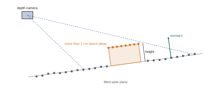
Planes dominate indoor and industrial scenes: floors, tables, walls, shelves and box faces. RANSAC (lesson 5) finds them robustly. Sample three points, compute the plane \( \mathbf{n} \cdot \mathbf{p} + d = 0 \) through them, count the points within a distance threshold, repeat, and refit the best plane to its inliers by least squares (the normal is the smallest-eigenvector direction of the inliers' covariance). Removing the dominant plane, the table or floor, is usually the first step in tabletop object detection: what remains above it are the objects. The same approach fits cylinders (pipes, cans), spheres and lines, and can be constrained, for example to planes whose normal is near vertical when looking for the floor.

import numpy as np
rng = np.random.default_rng(8)

fx = fy = 300.0; cx, cy = 160.0, 120.0
H, W = 240, 320
v, u = np.mgrid[0:H, 0:W]

# synthetic depth: a table plane tilted away from the camera, plus a box on top
Z = 0.9 + 0.0012 * (v - cy)                            # table depth rises toward the image bottom
box = (u > 130) & (u < 190) & (v > 90) & (v < 140)
Z = np.where(box, Z - 0.08, Z)                         # box top 8 cm closer to the camera
Z = Z + rng.normal(0, 0.002, Z.shape)                  # 2 mm noise
Z[rng.random(Z.shape) < 0.03] = 0.0                    # 3 % missing pixels

valid = Z > 0
X = (u - cx) * Z / fx; Y = (v - cy) * Z / fy
pts = np.column_stack([X[valid], Y[valid], Z[valid]])
lab = box[valid]
print("valid points:", len(pts))

# voxel downsample with 1 cm cubes
keys = np.floor(pts / 0.01).astype(int)
_, inv = np.unique(keys, axis=0, return_inverse=True)
cnt = np.bincount(inv.ravel())
vox = np.column_stack([np.bincount(inv.ravel(), pts[:, i]) / cnt for i in range(3)])
print("after 1 cm voxel grid:", len(vox))

# RANSAC plane
best_in = None
for _ in range(200):
    a, b, c = vox[rng.choice(len(vox), 3, replace=False)]
    n = np.cross(b - a, c - a)
    if np.linalg.norm(n) < 1e-9:
        continue
    n /= np.linalg.norm(n); d = -n @ a
    inl = np.abs(vox @ n + d) < 0.01
    if best_in is None or inl.sum() > best_in.sum():
        best_in = inl
P = vox[best_in]; centroid = P.mean(0)
n = np.linalg.svd(P - centroid)[2][-1]                 # least-squares refit
n = n if n[2] < 0 else -n                               # face the camera
d = -n @ centroid
print("table normal: (%.3f, %.3f, %.3f)" % tuple(n))
height = vox @ n + d                                    # signed height above the table
above = vox[height > 0.02]
print("voxels more than 2 cm above table:", len(above))
print("object height: %.3f m" % np.median(height[height > 0.02]))

valid points: 74574
after 1 cm voxel grid: 12156
table normal: (0.000, 0.359, -0.933)
voxels more than 2 cm above table: 544
object height: 0.068 m

The fitted normal shows the table tilted about 21° from facing the camera, and the voxels above it are the box. Its measured height, about 7 cm, is less than the 8 cm step in depth because the step was along the optical axis while height is measured perpendicular to the tilted table (8 cm × 0.93 ≈ 7.5 cm), and because voxels along the box edges mix box and table points. Reasoning about which direction a quantity is measured in is a constant habit in 3-D perception.

Clustering into objects

After the supporting plane is removed, the remaining points must be grouped into separate objects. Euclidean cluster extraction grows clusters by repeatedly adding neighbours within a distance threshold, using a k-d tree for fast neighbour search; clusters below a minimum size are discarded as noise. DBSCAN does the same with a density criterion. In organized clouds, connected-component labelling on the depth image with a depth-difference threshold is faster still. Each cluster then yields an oriented bounding box (from the principal axes of its points) or a centroid and extent, often enough for a simple grasp, or it can be passed to a recognition stage. Clustering fails when objects touch, which is where learned instance segmentation (lesson 10) helps.

Aligning point clouds

To merge views, track an object, or compare a scan with a CAD model, point clouds must be aligned. The iterative closest point (ICP) algorithm, introduced in ROB-310, alternates between pairing each point with its closest point in the other cloud and solving for the rigid transform that best aligns the pairs, which has a closed-form solution via SVD (the Kabsch method). Point-to-plane ICP, which minimizes distances along the target's normals, converges much faster on flat surfaces. ICP needs a good initial guess, because it converges to the nearest local minimum; global registration methods match local 3-D descriptors such as FPFH between the clouds and use RANSAC to find a rough alignment first.

Occupancy and free space

Mobile robots often convert depth data into simpler representations for navigation. A 2-D occupancy grid marks floor cells as free, occupied or unknown, built by projecting obstacle points down and ray-casting free space from the sensor to each measurement (ROB-340 covers mapping in depth). A 3-D voxel map such as an OctoMap stores occupancy probability in a hierarchical tree that adapts its resolution. For manipulation, signed distance fields and their truncated version (TSDF) fuse many depth frames into a smooth surface that collision checkers and planners can query. Whatever the representation, unknown space should be treated as potentially occupied: a depth camera that sees nothing over a dark or glass surface is not seeing empty space.