Visual odometry and structure from motion

A camera moving through the world sees the scene shift between frames, and that shift encodes both how the camera moved and where the scene points are. Visual odometry (VO) uses it to estimate the camera's motion frame by frame, like wheel odometry but without slipping wheels; structure from motion (SfM) recovers the camera poses and the 3-D structure together from a collection of images. VO runs on drones, planetary rovers (NASA's Mars rovers have used it since 2004), legged robots and phones, and it is the front end of the visual SLAM systems in ROB-340. This lesson assembles the pieces from lessons 2 to 6 into a working pipeline: matching, two-view motion from the essential matrix, triangulation, tracking against a growing map, and refinement by bundle adjustment.

The visual odometry pipeline

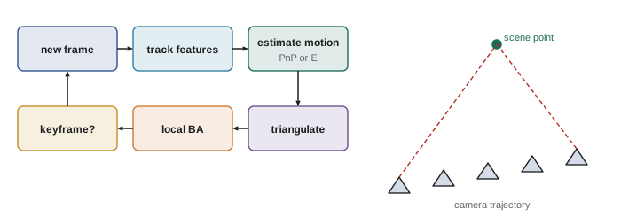
A typical feature-based monocular VO system repeats the same loop for each new frame.

1. Detect features (for example ORB or Shi–Tomasi corners) and match or track them from the previous frame. Tracking with the Lucas–Kanade optical-flow method, which follows each corner by minimizing brightness differences in a small window, is common at high frame rates because motion between frames is small.

2. Estimate the relative motion: with no map yet, from the essential matrix (five-point RANSAC); once 3-D points exist, from 2-D to 3-D matches with perspective-n-point (PnP, lesson 11), which is faster and more stable.

3. Triangulate new points seen in two or more frames to extend the map.

4. Periodically refine recent poses and points with local bundle adjustment.

5. Select keyframes: rather than keeping every frame, keep one when the camera has moved enough, or enough features have been lost, to add new information.

Direct methods such as DSO and semi-direct methods such as SVO skip explicit feature matching and instead minimize photometric error, the brightness difference between images warped by the estimated motion and depth. They use more of the image, including edges and weak texture, but need photometric calibration and are more sensitive to exposure changes. Feature-based methods such as ORB-SLAM's tracking front end are more tolerant of large motions and lighting changes.

Motion from two views

With calibrated cameras, the five-point algorithm inside RANSAC gives the essential matrix between two frames, and decomposing it gives the rotation R and the direction of the translation t, as lesson 6 explained. Two practical points matter. First, the estimate is poor when the translation is small relative to the scene depth, because the views then differ almost only by rotation and the translation direction is barely observable. VO systems wait for enough parallax, often measured as the median angle between corresponding rays, before initializing. Second, when the scene is nearly planar, the essential matrix becomes poorly determined, and a homography fits better; ORB-SLAM computes both and picks the model that explains the matches best.

import numpy as np
rng = np.random.default_rng(11)

def skew(t):
    return np.array([[0, -t[2], t[1]], [t[2], 0, -t[0]], [-t[1], t[0], 0]])

def rotz(a):
    c, s = np.cos(a), np.sin(a)
    return np.array([[c, -s, 0], [s, c, 0], [0, 0, 1]])

def roty(a):
    c, s = np.cos(a), np.sin(a)
    return np.array([[c, 0, s], [0, 1, 0], [-s, 0, c]])

# scene points 3-8 m ahead of camera 1; camera 2 moved and turned slightly
X = np.column_stack([rng.uniform(-2, 2, 60), rng.uniform(-1, 1, 60), rng.uniform(3, 8, 60)])
R_true = roty(np.deg2rad(5)) @ rotz(np.deg2rad(2))
t_true = np.array([0.5, 0.0, 0.1])                     # m, camera-2 frame
x1 = X / X[:, 2:]                                      # normalized coordinates
X2 = (R_true @ X.T).T + t_true
x2 = X2 / X2[:, 2:]
x1[:, :2] += rng.normal(0, 0.0005, (60, 2))           # about 0.5 px noise at f = 1000
x2[:, :2] += rng.normal(0, 0.0005, (60, 2))

# eight-point algorithm on all points, then enforce two equal singular values
A = np.array([np.kron(b, a) for a, b in zip(x1, x2)])
E = np.linalg.svd(A)[2][-1].reshape(3, 3)
U, S, Vt = np.linalg.svd(E)
E = U @ np.diag([1, 1, 0]) @ Vt

# decompose E into four candidates; keep the one with points in front of both cameras
U, _, Vt = np.linalg.svd(E)
if np.linalg.det(U) < 0: U = -U
if np.linalg.det(Vt) < 0: Vt = -Vt
Wm = np.array([[0, -1, 0], [1, 0, 0], [0, 0, 1]])
best = None
for R in (U @ Wm @ Vt, U @ Wm.T @ Vt):
    for t in (U[:, 2], -U[:, 2]):
        good = 0
        for a, b in zip(x1, x2):
            # solve z1 * R a + t = z2 * b for depths z1, z2 by least squares
            M = np.column_stack([R @ a, -b])
            z = np.linalg.lstsq(M, -t, rcond=None)[0]
            good += (z[0] > 0) and (z[1] > 0)
        if best is None or good > best[0]:
            best = (good, R, t)
good, R_est, t_est = best

ang = np.degrees(np.arccos(np.clip((np.trace(R_est.T @ R_true) - 1) / 2, -1, 1)))
tdir = np.degrees(np.arccos(abs(t_est @ t_true) / np.linalg.norm(t_true)))
print("points in front of both cameras: %d of 60" % good)
print("rotation error: %.3f deg" % ang)
print("translation direction error: %.2f deg" % tdir)
print("estimated |t| = %.2f (unit length: true scale %.2f m is unobservable)" % (np.linalg.norm(t_est), np.linalg.norm(t_true)))

points in front of both cameras: 60 of 60
rotation error: 0.225 deg
translation direction error: 1.12 deg
estimated |t| = 1.00 (unit length: true scale 0.51 m is unobservable)

Triangulation

Given the two camera poses and a matched pair of image points, the 3-D point lies where the two rays meet. With noise they never quite meet, so triangulation finds the point that best fits both. The linear method stacks the two projection equations into a small homogeneous system and solves it by SVD; the midpoint method takes the midpoint of the shortest segment between the rays; the optimal method minimizes reprojection error in both images. Triangulation accuracy depends on the angle between the rays, the parallax angle: depth uncertainty grows sharply as that angle shrinks, which is the same geometry as stereo depth error in lesson 6, with the distance travelled between frames acting as the baseline.

Scale and drift

A single camera cannot measure absolute scale: shrink the whole scene and the camera's motion by the same factor and every image is unchanged. Monocular VO therefore fixes the scale arbitrarily at initialization (say, the first translation has unit length) and carries it forward. Errors in triangulation then let the scale wander slowly, scale drift, so a monocular trajectory may be shaped correctly but grow or shrink over a long run. Scale is anchored with extra information: a stereo camera or depth sensor, wheel odometry, an IMU (visual-inertial odometry estimates scale from accelerometer readings, and is the norm on drones and phones), a known object size or the known height of the camera above a flat floor.

All odometry also drifts in position and heading, because each frame's small error is added to every later pose. Good stereo or visual-inertial odometry typically drifts about 0.5 % to 2 % of the distance travelled, depending on the environment and motion. Correcting that drift needs recognizing previously visited places and closing loops, which is the job of SLAM in ROB-340.

Bundle adjustment

VO's frame-to-frame estimates are locally consistent but not optimal. Bundle adjustment (BA) refines all camera poses and 3-D points together by minimizing the total reprojection error over every observation, the same objective as calibration in lesson 3 but with the cameras' poses and the points as unknowns:

where ρ is a robust loss to limit the influence of remaining outliers. The name refers to the bundles of rays from each camera, adjusted until they meet the points as well as possible. The problem is large (thousands of points and hundreds of cameras) but very sparse, because each point is seen by only a few cameras, and solvers such as Ceres, g2o and GTSAM exploit that sparsity with the Schur complement trick to eliminate the points and solve a small system for the cameras first. This is the same factor-graph optimization introduced in ROB-310, with reprojection factors. VO systems run local BA over a sliding window of recent keyframes in real time; offline SfM pipelines such as COLMAP run global BA over thousands of photos to build 3-D models.

Where visual odometry struggles

VO fails in predictable situations, and a robot should detect them rather than trust a bad estimate. Textureless surfaces such as white walls and smooth floors give too few features. Fast motion causes blur and large inter-frame displacement. Moving objects such as people, forklifts and doors violate the static-scene assumption unless rejected as outliers. Sudden lighting changes and auto-exposure jumps break brightness constancy for direct methods. Pure rotation gives no parallax for triangulation. Low light raises noise. The standard mitigations are an IMU to bridge short failures, global-shutter cameras with short exposures, a wider field of view, fixed exposure or photometric calibration, and monitoring of the number of tracked features and inliers to flag degraded tracking.