Epipolar geometry and stereo vision

One image loses depth; two images taken from different positions can recover it. Humans do this with two eyes a few centimetres apart, and robots do it with stereo cameras, which remain one of the most widely used depth sensors in mobile robotics, agriculture, automotive driver assistance and planetary exploration. Stereo works passively, in sunlight where many active depth sensors struggle, and its range scales with the baseline between the cameras. This lesson first develops epipolar geometry, the constraint that links any two views of a scene, and then specializes it to the rectified stereo pair, where depth comes from a single number per pixel, the disparity.

The epipolar constraint

Consider two cameras viewing the same point \( \mathbf{X} \). The two optical centres and the point define a plane, the epipolar plane. That plane cuts each image along a line, the epipolar line. The geometric consequence is powerful: if a point appears at \( \mathbf{u} \) in the first image, its match in the second image must lie somewhere on one known line. The search for a correspondence collapses from the whole image to a one-dimensional line.

All epipolar lines in an image pass through one point, the epipole, which is the image of the other camera's optical centre (it may lie far outside the image). When a camera moves straight forward, the epipole is the focus of expansion, the point from which the scene appears to stream outwards.

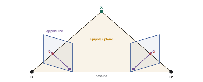
For calibrated cameras, write the motion from camera 1 to camera 2 as rotation R and translation t, and use normalized image coordinates \( \hat{\mathbf{x}} = K^{-1}\tilde{\mathbf{u}} \). The coplanarity of the two rays and the baseline gives the epipolar constraint

where \( [\mathbf{t}]_{\times} \) is the skew-symmetric cross-product matrix of t. E is the essential matrix, introduced by Longuet-Higgins in 1981. It has five degrees of freedom: three for rotation and two for the direction of translation, because the overall scale of t cannot be recovered from images alone. For uncalibrated pixel coordinates the same constraint holds with the fundamental matrix \( F = K_2^{-\mathsf{T}} E K_1^{-1} \), which has seven degrees of freedom. The epipolar line in image 2 for a point \( \tilde{\mathbf{u}}_1 \) is the vector \( \mathbf{l}_2 = F \tilde{\mathbf{u}}_1 \), with the line written as \( l_a u + l_b v + l_c = 0 \).

Estimating and decomposing the essential matrix

E can be estimated from point matches. Each match gives one linear equation in E's nine entries, so eight matches give a linear solution, the eight-point algorithm of Longuet-Higgins, made reliable by Hartley's 1997 normalization of coordinates. Nistér's five-point algorithm (2004) uses the minimal five matches and is the standard choice inside RANSAC for calibrated cameras. Once E is known, it can be decomposed into R and the direction of t; the decomposition gives four candidate solutions, and the correct one is the only one that places the triangulated points in front of both cameras. Lesson 7 uses exactly this to compute camera motion.

The rectified stereo pair

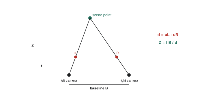
A stereo camera makes the geometry as simple as possible. Its two cameras are mounted side by side with parallel optical axes, separated by a baseline B, and after calibration both images are rectified: warped so that their image planes are coplanar and their rows aligned. Then every epipolar line is a horizontal row, and a point at row v in the left image appears on row v in the right image too. The only difference is a horizontal shift, the disparity

By similar triangles, depth follows directly from disparity:

where f is the focal length in pixels. Near objects have large disparities and far objects small ones, approaching zero at infinity. Rectification uses the stereo calibration (the intrinsics of both cameras and the rotation and translation between them, found as in lesson 3 from simultaneous views of a target) to compute a rectifying rotation for each camera; OpenCV's stereoRectify and the ROS stereo_image_proc package do this routinely.

How depth error grows with distance

Differentiating \( Z = fB/d \) with respect to d shows how a disparity error \( \delta d \) becomes a depth error:

Depth error grows with the square of distance. This is the single most important fact about stereo: a sensor accurate to a few millimetres at 1 m may be uncertain by tens of centimetres at 10 m. It is also the design rule. A longer baseline or longer focal length reduces error at a given range but increases the minimum range (because near points leave one camera's view or exceed the disparity search range) and narrows the field of view. Disparity can be estimated to a fraction of a pixel with sub-pixel interpolation, typically 0.1 to 0.25 px in good texture.

Computing disparity: stereo matching

Finding the disparity for every pixel, dense stereo matching, means finding, for each left-image pixel, the best-matching position along the same row of the right image within a disparity range \( [0, d_{max}] \). Local methods compare small windows using a cost such as the sum of absolute differences (SAD), the sum of squared differences, normalized cross-correlation, or the census transform, which compares bit patterns of local brightness orderings and is robust to exposure differences between the cameras. The disparity with the lowest cost wins.

Local matching fails where windows are ambiguous: textureless walls, repetitive patterns, and occluded regions that one camera sees and the other does not. Global and semi-global methods add a smoothness term that penalizes disparity jumps between neighbours except at strong image edges. Semi-global matching (SGM, Hirschmüller, 2005) approximates this efficiently by aggregating costs along several directions, and it runs in real time on embedded hardware; it is the basis of many commercial stereo cameras. A left-right consistency check (match right to left as well and reject pixels whose disparities disagree) removes most occlusion errors. Learned stereo networks now produce the most accurate disparity maps on benchmarks, at higher computational cost.

import numpy as np
rng = np.random.default_rng(5)

H, W, dmax, win = 40, 120, 24, 5
left = rng.integers(0, 255, (H, W)).astype(float)       # random texture
true_d = np.full((H, W), 6)                              # background at disparity 6
true_d[10:30, 50:90] = 18                                # nearer box at disparity 18
right = np.zeros_like(left)
for v in range(H):
    for u in range(W):
        src = u + true_d[v, u]                           # right pixel u sees left pixel u + d
        right[v, u] = left[v, src] if src < W else rng.integers(0, 255)
right += rng.normal(0, 4, right.shape)                   # sensor noise

# shift-and-compare: right view displaced to line up with the left
hw = win // 2
best_cost = np.full((H, W), np.inf)
disp = np.zeros((H, W), int)
k = np.ones(win) / win
for d in range(dmax + 1):
    shifted = np.full_like(right, 1e6)
    shifted[:, d:] = right[:, :W - d]
    cost = np.abs(left - shifted)
    cost = np.apply_along_axis(lambda r: np.convolve(r, k, 'same'), 1, cost)   # box sum along rows
    cost = np.apply_along_axis(lambda c: np.convolve(c, k, 'same'), 0, cost)   # and columns
    better = cost < best_cost
    best_cost[better] = cost[better]
    disp[better] = d

inner = (slice(hw, H - hw), slice(dmax + hw, W - hw))
acc = (disp[inner] == true_d[inner]).mean()
print("pixels with correct disparity: %.1f %%" % (100 * acc))
print("median disparity on the box: %d (true 18)" % np.median(disp[12:28, 55:85]))
f, B = 700, 0.12
print("box depth: %.2f m, background depth: %.2f m" % (f * B / 18, f * B / 6))

pixels with correct disparity: 82.9 %
median disparity on the box: 18 (true 18)
box depth: 4.67 m, background depth: 14.00 m

Note that the reference image is the left one and the matching pixel in the right image lies at \( u - d \); the code expresses this by shifting the right image d pixels to the right before comparing. Errors concentrate at the box edges, where one camera sees background that the other cannot.

Stereo in practice

Off-the-shelf stereo cameras integrate the cameras, calibration and a matching processor and output a depth image directly (ROB-220 compared them with structured light and time-of-flight sensors). Some add an infrared pattern projector to give texture to blank walls indoors, while still working passively in sunlight. When choosing or using one, check the baseline and focal length against the required range accuracy using \( \delta Z = Z^2 \delta d/(fB) \); check the minimum range; synchronize the two exposures (unsynchronized rolling-shutter cameras give false disparities on moving objects); and expect holes in the depth image on textureless, shiny, transparent and very dark surfaces.