Learning-based perception I: classification and convolutional networks

The methods in lessons 4 to 8 are designed by hand: an engineer decides that corners matter and writes a formula to find them. That works well for geometry, but recognizing what something is, a ripe strawberry, a damaged parcel, a person stepping into an aisle, depends on appearance in ways too varied to write down. Since 2012, when a convolutional neural network called AlexNet cut the error rate of the ImageNet image-classification benchmark nearly in half, learned models have dominated recognition. Robots now use them for classification, detection, segmentation, depth, keypoints and even direct control. This lesson explains how convolutional networks work, how they are trained and evaluated, and what a robotics engineer needs to know to use them responsibly. Lesson 10 builds on it for detection and segmentation.

From features to learned features

A classifier maps an input, here an image, to one of K classes. The classical approach computes hand-designed features (colour histograms, gradient histograms such as HOG, SIFT descriptors pooled into a 'bag of words') and trains a simple classifier on them, such as a support vector machine. Deep learning instead learns the features and the classifier together from labelled examples, by adjusting millions of parameters to reduce a loss function. Given enough representative data, learned features consistently outperform hand-designed ones on recognition, and they adapt to whatever the task needs.

The building block is the artificial neuron: a weighted sum of inputs plus a bias, passed through a non-linear activation function. The most common activation is the rectified linear unit, \( \text{ReLU}(x) = \max(0, x) \), which is cheap and keeps gradients from vanishing in deep networks. Layers of neurons stacked in sequence form a network; without the non-linearities, any stack of linear layers would collapse to a single linear map.

Convolutional layers

A fully connected layer joins every input to every output, which is wasteful for images: a 224 × 224 × 3 input connected to just 1,000 neurons needs 150 million weights. Convolutional layers exploit two properties of images. Locality: nearby pixels are related, so each output looks only at a small window. Translation equivariance: a pattern means the same thing wherever it appears, so the same weights are applied at every position. A convolutional layer is therefore a bank of learned filters, exactly the kernels of lesson 4, except that the network chooses their weights. Each filter spans all input channels and produces one output channel, a feature map.

For an input of width W, kernel size k, padding p and stride s, the output width is

and a layer with \( C_{in} \) input channels and \( C_{out} \) filters of size k × k has \( (k^2 C_{in} + 1)\,C_{out} \) parameters, independent of image size. Pooling layers (for example 2 × 2 max pooling) or strided convolutions halve the resolution between stages, so deeper layers see larger regions of the image, their receptive field, and respond to larger, more abstract patterns. Early layers learn edge and colour detectors very like Gabor filters; middle layers respond to textures and parts; late layers respond to whole objects. A final global average pool and fully connected layer produce one score per class, and the softmax function turns scores \( z_k \) into probabilities:

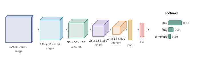
Important architectures include VGG (2014), ResNet (2015), whose residual skip connections made networks of 50 to 150 layers trainable, MobileNet and EfficientNet, designed for phones and embedded robots, and vision transformers (ViT, 2020), which split the image into patches and use attention instead of convolution. At the time of writing, both convolutional and transformer backbones are in wide use, and large self-supervised backbones such as DINOv2 provide general-purpose features that work well with little task-specific data.

Training

Training adjusts the parameters θ to minimize a loss averaged over labelled examples. For classification the loss is the cross-entropy between the predicted probabilities and the true class y, \( L = -\log p_y \): near zero when the network is confidently right and large when it is confidently wrong. Backpropagation computes the gradient of the loss with respect to every parameter by the chain rule, and stochastic gradient descent (or a variant such as Adam) takes a small step against it on a random mini-batch of examples, repeating for many passes (epochs) through the data.

The central danger is overfitting: a large network can memorize its training images and still fail on new ones. The defences are standard practice.

• Split the data into training, validation and test sets, with the test set touched only once at the end. Split by scene, robot run or day, not by random frame, because consecutive video frames are nearly identical and leak information between sets.
• Data augmentation: random crops, flips, rotations, colour jitter, blur and noise teach invariance to changes the robot will meet.
• Regularization: weight decay, dropout and early stopping when validation loss stops improving.
• Transfer learning: start from a backbone pre-trained on a large dataset and fine-tune on the task. A few hundred labelled images per class often suffice this way, versus hundreds of thousands from scratch.

import numpy as np
rng = np.random.default_rng(4)

def make(n):
    """8 x 8 images: class 1 has a vertical bar (a 'pin'), class 0 a horizontal bar, with noise."""
    X = rng.normal(0, 0.35, (n, 8, 8)); y = rng.integers(0, 2, n)
    for i in range(n):
        k = rng.integers(1, 7)
        if y[i]: X[i, :, k] += 1.0
        else:    X[i, k, :] += 1.0
    return X.reshape(n, 64), y

Xtr, ytr = make(600); Xte, yte = make(400)

# one learned 'filter' per pixel: logistic regression trained by gradient descent
w = np.zeros(64); b = 0.0; lr = 0.1
for epoch in range(300):
    p = 1 / (1 + np.exp(-(Xtr @ w + b)))
    g = p - ytr                                  # gradient of cross-entropy w.r.t. scores
    w -= lr * Xtr.T @ g / len(ytr); b -= lr * g.mean()

def evaluate(X, y):
    pred = (1 / (1 + np.exp(-(X @ w + b)))) > 0.5
    tp = int(((pred == 1) & (y == 1)).sum()); fp = int(((pred == 1) & (y == 0)).sum())
    fn = int(((pred == 0) & (y == 1)).sum()); tn = int(((pred == 0) & (y == 0)).sum())
    return tp, fp, fn, tn

tp, fp, fn, tn = evaluate(Xte, yte)
print("test confusion: TP=%d FP=%d FN=%d TN=%d" % (tp, fp, fn, tn))
print("accuracy %.3f, precision %.3f, recall %.3f" % ((tp + tn) / len(yte), tp / (tp + fp), tp / (tp + fn)))
Wimg = w.reshape(8, 8)
print("mean weight, top and bottom rows (cols 1-6): %+.3f" % Wimg[[0, 7], 1:7].mean())
print("mean weight, left and right columns (rows 1-6): %+.3f" % Wimg[1:7, [0, 7]].mean())
print("mean weight, interior pixels: %+.3f" % Wimg[1:7, 1:7].mean())

test confusion: TP=164 FP=22 FN=34 TN=180
accuracy 0.860, precision 0.882, recall 0.828
mean weight, top and bottom rows (cols 1-6): +0.569
mean weight, left and right columns (rows 1-6): -0.604
mean weight, interior pixels: +0.008

The weights reveal how this simple model decides. Because bars never sit on the outer rows or columns, a vertical bar always reaches the top and bottom edges and a horizontal bar always reaches the left and right edges. The model learned to look there, with positive weights on the top and bottom rows and negative weights on the side columns, rather than recognizing 'bar-ness' everywhere. That is a small example of shortcut learning: networks exploit whatever pattern separates the training classes, which may not be the pattern the engineer intended. A real camera image of a pin cropped differently would fool it, which is exactly why test data must come from conditions the robot will really meet. A convolutional network with several filters and pooling would instead learn local oriented-bar detectors that work anywhere in the image.

Measuring performance

Accuracy, the fraction classified correctly, is misleading when classes are unbalanced or errors have different costs, which is almost always true in robotics. A safety classifier that never reports a person in an aisle that is empty 99 % of the time is 99 % accurate and useless. Use the confusion matrix and the measures built from it:

Precision asks what fraction of positive reports were right; recall asks what fraction of real positives were found. Raising the decision threshold usually trades recall for precision, and the right operating point depends on cost: a weed-spraying robot might prefer high precision (do not spray crops), while a person detector for a safety stop needs very high recall (never miss a person), accepting some false stops. The F1 score, the harmonic mean of the two, summarizes both. Calibration also matters: a network's softmax output of 0.9 is often not a 90 % probability of being right, and techniques such as temperature scaling can correct it so downstream decisions can use the confidence meaningfully.

Using learned models on robots

Deploying a network on a robot raises engineering questions beyond accuracy. Inference must fit the latency budget of ROB-320 on the available hardware: an embedded GPU module, a neural accelerator or a CPU. Models are typically exported to ONNX and optimized with tools such as TensorRT or OpenVINO, often with 8-bit integer quantization that cuts memory and time by two to four times for a small accuracy loss. Inputs must be pre-processed exactly as in training: the same resizing, normalization and colour order (RGB versus BGR is a classic bug). And the robot's environment will differ from the training data, a problem called distribution shift: new lighting, new products, dirty lenses, seasons. Monitoring confidence, logging hard cases, and periodically retraining on data from the field are part of operating a learned perception system, as is keeping a non-learned safety layer, such as a certified safety scanner, for functions where a missed detection could injure someone.