
SLS-214 · Lesson 7 of 12 · 25 min
Forecasting with a weighted pipeline
▶ Video coming soon A video version of this lesson is on the way.
By October 30, Rob's question from the first session had become urgent. Ridgeline's fiscal year would end in a month, and the leadership team wanted a forecast for the fourth quarter that it could give to the owners. Grace said she would build two forecasts and compare them. The first, covered in this lesson, would be mechanical: a weighted pipeline built straight from the CRM. The second, in lesson 8, would add the sellers' and managers' judgment. "The mechanical forecast is honest but naive," she said. "Judgment is informed but optimistic. We need both."
A sales forecast is an estimate of the bookings a seller, team or company will achieve in a period. Forecasts are used to plan hiring, inventory, cash and production, and to set expectations with owners and lenders. A forecast that is consistently too high or too low causes real problems: Ridgeline had once hired two installers for a winter rush that did not come.
Stage probabilities
A weighted pipeline gives every open opportunity a probability, usually based on its stage, and multiplies its value by that probability. The sum of these weighted values is the forecast. Ridgeline's CRM assigned these default probabilities.
| Stage | Default probability |
|---|---|
| Qualify | 10 in 100 |
| Discover | 25 in 100 |
| Propose | 50 in 100 |
| Negotiate | 75 in 100 |
| Closed Won | 100 in 100 |
| Closed Lost | 0 |
The symbol Σ means "add up over all the opportunities". In a spreadsheet, the same calculation is one formula. If the values are in column C and the probabilities in column D, then =SUMPRODUCT(C2:C8, D2:D8) multiplies each pair and adds the results.
Worked problem
Maya's weighted pipeline
On November 13, Maya has seven open opportunities with these total contract values and stages: Westgate & Rowe 13,800 (Propose), Eastgate Physiotherapy 14,400 (Propose), Northfield's expansion 18,080 (Propose), Keystone's training centre 48,000 (Negotiate), Harvest Valley Credit Union 34,800 (Discover), Bellmont Seniors Residence 27,800 (Qualify) and Sandstone Accounting 16,500 (Qualify). Calculate her total pipeline and her weighted pipeline.
Show solution
- Total pipeline.
- \[13{,}800 + 14{,}400 + 18{,}080 + 48{,}000 + 34{,}800 + 27{,}800 + 16{,}500 = 173{,}380\]
- Propose: three deals totalling 46,280 dollars at 0.50.
- \[46{,}280 \times 0.50 = 23{,}140\]
- Negotiate: 48,000 at 0.75.
- \[48{,}000 \times 0.75 = 36{,}000\]
- Discover: 34,800 at 0.25.
- \[34{,}800 \times 0.25 = 8{,}700\]
- Qualify: two deals totalling 44,300 at 0.10.
- \[44{,}300 \times 0.10 = 4{,}430\]
- Add the weighted values.
- \[23{,}140 + 36{,}000 + 8{,}700 + 4{,}430 = 72{,}270\]
Answer: Maya's pipeline is 173,380 dollars of total contract value, and her weighted pipeline is 72,270 dollars. The weighted figure is a rough estimate of how much contract value these seven deals will eventually produce, whenever they close.
| A: Opportunity | B: Stage | C: Value | D: Probability | E: Weighted | |
|---|---|---|---|---|---|
| 2 | Westgate & Rowe | Propose | 13,800 | 0.50 | =C2*D2 → 6,900 |
| 3 | Eastgate Physiotherapy | Propose | 14,400 | 0.50 | =C3*D3 → 7,200 |
| 4 | Northfield expansion | Propose | 18,080 | 0.50 | =C4*D4 → 9,040 |
| 5 | Keystone training centre | Negotiate | 48,000 | 0.75 | =C5*D5 → 36,000 |
| 6 | Harvest Valley CU | Discover | 34,800 | 0.25 | =C6*D6 → 8,700 |
| 7 | Bellmont Seniors | Qualify | 27,800 | 0.10 | =C7*D7 → 2,780 |
| 8 | Sandstone Accounting | Qualify | 16,500 | 0.10 | =C8*D8 → 1,650 |
| 9 | Total | =SUM(C2:C8) → 173,380 | =SUMPRODUCT(C2:C8,D2:D8) → 72,270 |
This figure is not yet a forecast for any period, because it ignores close dates. Keystone's training centre is not expected until January, Bellmont until March and Sandstone until May. A forecast for a period must include only the deals expected to close in it.
The fourth-quarter forecast
For the leadership team, Grace built the weighted forecast for the five established account executives and the Prairie Valley house account, using first-year value, because that is what the fiscal-year target measures, and including only opportunities with a close date on or before November 30.
Worked problem
Weighted forecast for the quarter
By November 13 the team has booked 512,000 dollars in the fourth quarter. Open opportunities with close dates by November 30 have these first-year values: Qualify 40,000, Discover 118,000, Propose 386,000 and Negotiate 264,000 dollars, which includes Prairie Valley's 66,000. Calculate the weighted forecast for the rest of the quarter, the forecast for the quarter, and the forecast for the year against the 3,000,000-dollar annual quota. The team booked 2,036,000 dollars in the first three quarters.
Show solution
- Weight each stage.
- \[40{,}000 \times 0.10 = 4{,}000\]
- \[118{,}000 \times 0.25 = 29{,}500\]
- \[386{,}000 \times 0.50 = 193{,}000\]
- \[264{,}000 \times 0.75 = 198{,}000\]
- \[4{,}000 + 29{,}500 + 193{,}000 + 198{,}000 = 424{,}500\]
- Add what is already booked.
- \[512{,}000 + 424{,}500 = 936{,}500\]
- Add the first three quarters.
- \[2{,}036{,}000 + 936{,}500 = 2{,}972{,}500\]
- \[\frac{2{,}972{,}500}{3{,}000{,}000} \approx 0.991\]
Answer: The weighted forecast for the quarter is 936,500 dollars, just short of the 964,000 dollars needed. The forecast for the year is 2,972,500 dollars, about 99.1 in 100 of quota.
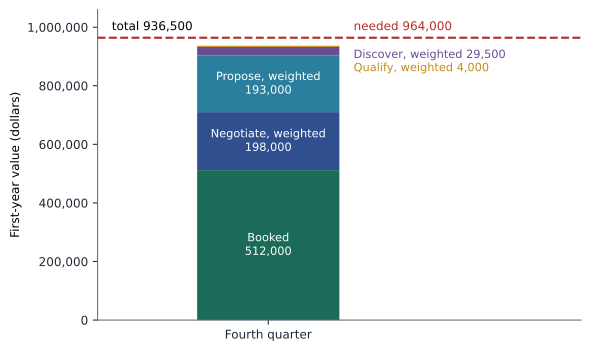
Rob looked at the number and asked the right question: "How much of that 424,500 is real?" The weighted forecast had three well-known weaknesses, and Grace explained each one.
Weakness 1: probabilities that do not match history
Default probabilities like 10, 25, 50 and 75 are round numbers chosen by someone, not measured. A better approach is to set them from history: of the opportunities that reached each stage, what share were eventually won? Lesson 3's second-quarter cohort gives the answer.
| Stage reached | Opportunities | Eventually won | Historical win probability | Default |
|---|---|---|---|---|
| Qualify | 120 | 27 | 27 ÷ 120 = 22.5 in 100 | 10 in 100 |
| Discover | 84 | 27 | 27 ÷ 84 = 32.1 in 100 | 25 in 100 |
| Propose | 57 | 27 | 27 ÷ 57 = 47.4 in 100 | 50 in 100 |
| Negotiate | 38 | 27 | 27 ÷ 38 = 71.1 in 100 | 75 in 100 |
The defaults were close for the later stages and too low for the early ones. But there is a second issue: the historical probability says whether a deal is eventually won, not whether it is won within the next 17 days. A deal in Qualify on November 13 will almost never close by November 30, because Ridgeline's median cycle is about two months. Grace's rule for quarter-end forecasts was to give early-stage deals little or no weight unless the seller could show a specific reason they would close in time. This is called calibrating the probabilities: adjusting them so that, over many deals, the forecast matches what actually happens.
Weakness 2: lumpy deals
A weighted pipeline treats a 75 in 100 deal worth 66,000 dollars as if it will produce 49,500 dollars. It will not. Prairie Valley will either sign, adding 66,000 dollars, or not sign this quarter, adding nothing. When a forecast contains a few large deals, the weighted total can be a number that no actual outcome produces. With dozens of similar deals the averages work out; with a handful of large ones, they do not.
Grace handled lumpy deals separately. She took the largest deals out of the weighted calculation and showed each one as a yes or no with a stated likelihood. For the fourth quarter that meant showing Prairie Valley on its own: the weighted forecast without it, and the forecast if it signed.
Worked problem
Separating the large deal
Remove Prairie Valley (66,000 dollars at 75 in 100) from the Negotiate total and recalculate the quarter's forecast with and without the contract signed.
Show solution
- Negotiate without Prairie Valley.
- \[264{,}000 - 66{,}000 = 198{,}000\]
- \[198{,}000 \times 0.75 = 148{,}500\]
- Weighted forecast for the other deals.
- \[4{,}000 + 29{,}500 + 193{,}000 + 148{,}500 = 375{,}000\]
- Quarter forecast without Prairie Valley.
- \[512{,}000 + 375{,}000 = 887{,}000\]
- Quarter forecast with Prairie Valley signed.
- \[887{,}000 + 66{,}000 = 953{,}000\]
Answer: Without Prairie Valley, the quarter forecast is 887,000 dollars; with it, 953,000. Neither reaches 964,000, so making the year needs Prairie Valley and some additional business.
Weakness 3: bad data
A weighted pipeline is only as good as the stages and close dates in the CRM. Sellers often leave close dates at the end of the current quarter out of optimism, and move them forward when the quarter ends. Grace counted how often this had happened.
Worked problem
Slipped close dates
Of the 46 opportunities that had close dates in the third quarter on July 1 and were still open on August 31, 29 had their close date moved into the fourth quarter. What share slipped?
Show solution
- \[\frac{29}{46} \approx 0.630\]
Answer: About 63 in 100 of the deals still open at the end of the quarter had simply been pushed into the next one. That is a sign that close dates were optimistic, and it means the fourth-quarter pipeline contained deals that had already slipped once.
Deals that have slipped once are more likely to slip again. Some forecasting methods reduce the probability of a deal each time its close date moves. Grace preferred a simpler step: she flagged every opportunity that had slipped and asked its owner, in the forecast meeting, what had changed. That brought judgment into the forecast, which is the subject of lesson 8.
When weighted pipeline works well
Despite its weaknesses, the weighted pipeline is valuable. It is objective: it does not depend on anyone's mood. It is quick, because the CRM calculates it automatically. It treats every seller the same way, so it is a useful check on the more optimistic sellers. And it works well for teams with many similar, moderately sized deals and well-maintained data. Grace used it as a baseline that the judgment-based forecast had to explain any difference from.
Checking the weighted forecast after the fact
A forecasting method earns trust by being checked. At the end of each quarter, Grace compared the weighted forecast she had made two weeks before quarter end with actual bookings, and she also checked the probabilities themselves: of all the deals that had been in Negotiate two weeks before the end, what share had actually closed in the quarter? If the answer was well below 75 in 100, the Negotiate probability was too high for quarter-end forecasting, even if it was right for eventual wins.
She kept these checks in a simple table with one row per quarter. Over the first three quarters of fiscal 2026, Negotiate deals two weeks out had closed in the quarter about 64 times in 100, Propose deals about 31 times in 100, and Discover deals almost never. Those figures, rather than the CRM defaults, became the probabilities she used for her quarter-end weighted forecast from December. The defaults stayed in the CRM for long-range pipeline views, where eventual win probability is what matters.
Worked problem
A forecast with quarter-end probabilities
Using quarter-end probabilities of 64 in 100 for Negotiate, 31 in 100 for Propose and zero for earlier stages, recalculate the weighted forecast for the team's fourth-quarter deals other than Prairie Valley: 198,000 dollars in Negotiate and 386,000 dollars in Propose.
Show solution
- \[198{,}000 \times 0.64 = 126{,}720\]
- \[386{,}000 \times 0.31 = 119{,}660\]
- \[126{,}720 + 119{,}660 = 246{,}380\]
- Add the 512,000 dollars already booked.
- \[512{,}000 + 246{,}380 = 758{,}380\]
Answer: About 758,380 dollars for the quarter without Prairie Valley, or about 824,380 with it, much closer to the sellers' judgment in lesson 8 than the default-probability figure of 887,000.
Some CRMs now offer forecasts produced by machine-learning models that look at many signals at once, such as how recently the customer replied, how many people are involved and how long the deal has been in its stage. Grace treated these as a third opinion rather than a replacement. They were useful for spotting deals that looked risky, but their reasoning was hard to explain to the owners, and they learned from Ridgeline's own history, including its old habit of optimistic close dates.
Common mistakes
MistakeForecasting a period from all open pipeline regardless of close date.
InsteadInclude only opportunities expected to close in the period.
MistakeUsing round default probabilities without checking history.
InsteadCalibrate stage probabilities against how often deals at each stage were actually won.
MistakeGiving early-stage deals weight in a quarter that ends in two weeks.
InsteadWeight deals by their chance of closing in the period, not eventually.
MistakeTreating a weighted large deal as partial revenue.
InsteadShow large deals separately as yes or no.
MistakeTrusting close dates that have slipped.
InsteadFlag slipped deals and ask what has changed.
Summary and key terms
- A weighted pipeline multiplies each open opportunity's value by its stage probability and adds them; in a spreadsheet, =SUMPRODUCT(values, probabilities).
- Maya's 173,380 dollars of pipeline weighted to 72,270, but a forecast for a period includes only deals expected to close in it.
- The team's fourth-quarter weighted forecast was 936,500 dollars, about 99.1 in 100 of the annual quota.
- Three weaknesses need care: default probabilities should be calibrated against history and against the time left; large deals are lumpy and should be shown separately as yes or no (887,000 without Prairie Valley, 953,000 with it); and slipped close dates make the pipeline optimistic.
- The weighted pipeline is an objective baseline.
- Sales forecast
- An estimate of the bookings a seller, team or company will achieve in a period.
- Weighted pipeline
- The sum of each open opportunity's value multiplied by its probability.
- Stage probability
- The likelihood assigned to an opportunity based on its stage.
- Calibration
- Adjusting probabilities so that forecasts match actual outcomes over many deals.
- Lumpy deal
- A deal large enough that its yes-or-no outcome swings the forecast.
- Slippage
- Moving an opportunity's close date later, often into the next period.
Practice problems
Work each problem on paper first, then reveal the answer to check.
Three deals worth 10,000, 20,000 and 30,000 dollars have probabilities of 0.25, 0.50 and 0.75. What is the weighted pipeline?
Show answer
2,500 + 10,000 + 22,500 = 35,000 dollars.
Of 90 opportunities that reached Propose, 45 were won. What is the historical win probability from Propose?
Show answer
45 ÷ 90 = 0.50, or 50 in 100.
Why show a very large deal separately?
Show answer
Its outcome is all or nothing, so a weighted share of it is not a realistic result.
Lesson quiz · 5 questions
Score 60% or more to complete this lesson.
Create a free account to save your progress, take quizzes and earn a certificate.